The periodic responses and quasi-periodic motions of a van der Pol-Mathieu equation subjected to three excitations, i.e., self-excited, parametric excitation, and external excitation, are studied in this paper. A new characteristic is observed that the spectra of the quasi-periodic motions contain uniformly spaced sideband frequencies. Firstly, the traditional incremental harmonic balance (IHB) method is used to obtain periodic responses of the van der Pol-Mathieu equation and to trace their nonlinear frequency response curves automaically. Then the Floquet theory is used to analyze stability of the periodic responses and their bifurcations. Based on the characteristic that the spectra of quasi-periodic motions contain two incommensurate basic frequencies, i.e., the excitation frequency and a priori unknown frequency related to uniformly spaced sideband frequencies. Then the IHB method with two time-scales basing on the two basic frequencies is formulated to accurately calculate all frequency components and their corresponding amplitudes even at critical points. All the results obtained from the IHB method with two time-scales are in excellent agreement with those from numerical integration using the fourth-order Runge-Kutta method. Finally, this investigation reveals rich dynamic characteristics of the van der Pol-Mathieu equation in a range of excitation frequencies.
Keywords:van der Pol-Mathieu equation
;
incremental harmonic balance method with two time-scales
;
bifurcation
;
quasi-periodic motion
;
sideband
Huang Jianliang, Wang Teng, Chen Shuhui. NONLINEAR DYNAMIC ANALYSIS OF A VAN DER POL-MATHIEU EQUATION WITH EXTERNAL EXCITATION1). Chinese Journal of Theoretical and Applied Mechanics[J], 2021, 53(2): 496-510 DOI:10.6052/0459-1879-20-310
引言
在工程中存在着很多可以用自激振动和参数激振联合作用的van der Pol-Mathieu方程来描述的振动, 例如, 含有万向接头的转子系统的横向振动[1], 卡盘作业过程中的参数激振[2], 含有自振和参数激振的齿轮装置系统的振动[3], 尘埃等离子体中的颗粒电荷的动力学行为[4], 高层建筑结构在风荷载下的振动[5-6]等, 都是可用van der Pol-Mathieu方程来描述振动的典型例子. van der Pol-Mathieu方程同时含有自激振动和参数激振, 蕴含着丰富的动力学行为, 多年来一直是众多学者关注点之一.
Tondl[7]首先分析了van der Pol-Mathieu方程中自激振动和参数激振的相互作用, 并在共振区域发现了周期响应. Kotera和Yano[8]用两个频率的和分析了van der Pol-Mathieu方程在参数共振区域的近似一阶和二阶的周期解. 陈予恕和徐鉴[9]研究了van der Pol-Duffing-Mathieu型系统主参数共振分岔解, 得到该非线性参数激励系统依赖于物理参数变化的振动模式. Szabelski和Warminski[10]分析了自激振动和参数激励对van der Pol-Mathieu方程的影响, 并且研究了附加外激励在同步区域内动力学行为的影响. Warminski等[3]对含有自激振动和参数激励的两自由度系统进行分析, 并得到了不同类型的响应, 包含有周期响应, 准周期运动响应和混沌. 彭献和陈自力[11]引入参数变换, 将强非线性系统转化为弱非线性系统, 利用摄动思想分析得到了van der Pol-Mathieu方程的1/2亚谐共振周期解. Belhaq和Fahsi[12]和Pandey等[13]分析了van der Pol-Mathieu-Duffing系统的响应, 得到该类系统可含有1:1锁频, 2:1次谐波锁频和准周期运动响应. 张琪昌等[14]利用改进的类Padé方法计算了van der Pol-Duffing方程的同异宿轨道. Warminski[15]研究了含有van der Pol和Rayleigh函数在两个不同自激振动模型下具有时滞状态的自激振动, 参数激振和强迫振动作用下的相互作用. 许多学者也对各类含有参数激振的非线性系统进行研究[16-19], 得到了不同的非线性振动特性和运动分岔.
早期对于van der Pol-Mathieu方程的众多研究主要集中在含有一个基频的周期响应及其稳定性分析. 可以利用不同的摄动方法求得这类方程的近似解析解[20]. 然而, 对于van der Pol-Mathieu方程来说, 因有自激振动与参数激励振动的相互耦合作用, 使得系统不仅有周期响应, 而且还有准周期运动响应, 甚至产生混沌, 近年来受到众多学者的关注. Belhaq和Houssni[21]为了构造准周期运动的近似解, 提出了双摄动的思想, 其方法包含了两个步骤: 第一步利用广义的平均法将准周期系统变为周期减化系统; 第二步是用多尺度法对周期减化系统构造出近似的准周期运动解. 他们利用双摄动方法得到了同时含有二次和三次非线性项的参数激励和外激励的单自由度系统的准周期解. 该双摄动方法的本质就是对周期减化系统在平衡点附近的周期解进行非线性近似, 该方法可进一步推广到各类非线性系统的准周期运动分析中[5-6,12,22]. Fan等[23]也利用了双摄动方法分析了van der Pol-Mathieu方程在有外激励和无外激励两种情况下的周期解和准周期运动近似解的包络线. 然而, 双摄动方法只能得到准周期运动包络线的最大和最小幅值, 无法得到系统准周期运动的具体响应情况, 更无法得到系统准周期运动的各个响应频率. Warminski等[3]和Warminski[15]利用多尺度法分别分析了含有自激励和参数激励的两个自由度时滞系统, 并利用数值法得到了两个时滞系统的准周期运动响应和混沌. Veerman和Verhulst[24]利用平均法分析了van der Pol-Mathieu方程, 并得到了由1阶和1/$\varepsilon$阶基础周期构造而成的准周期运动响应, 其中$\varepsilon$是小量. 上述的各种摄动法只能得到van der Pol-Mathieu方程准周期运动近似解, 有些方法得到的结果只能描述准周期运动的最大和最小振幅, 特别是在邻近分岔点处用摄动法得到的准周期运动解与数值解相差甚大, 据作者所知, 迄今为止尚未有有效的摄动法能精确地计算并得到此类van der Pol-Mathieu方程的精确准周期运动解.
本文针对含有外激励的van der Pol-Mathieu方程进行研究, 主要是发现了单自由度的van der Pol-Mathieu方程准周期运动的频谱含有均匀边频带的新特性。 此新特性与之前研究分析的多自由度非线性系统中内共振引起的准周期运动的频谱特性[25-27]相类似, 即都含有均匀的边频带, 不同之处在于多自由度非线性系统中的准周期运动是由于不同振动模态之间在内共振条件下相互作用产生的, 而单自由度的van der Pol-Mathieu方程的准周期运动是由于自激振动与参数激振耦合产生的, 仅是van der Pol方程中的自激振动或仅是Mathieu方程中的参数激振并不能产生准周期运动. 根据此准周期运动频谱含有均匀边频带的特性, 它包含了两个基频, 一个是已知激励频率$\omega$; 另一个是事先未知的频率$\omega_{\rm d}$, 即为边频带中相邻两个频率之间的距离, 那么准周期运动中所有的频率成份都可表示为这两个基频的线性组合. 因此, 本文利用传统的增量谐波平衡法(IHB法)分析单自由度含有外激励的van der Pol-Mathieu方程的周期响应, 并推广两时间尺度的IHB法, 其中一个时间尺度是快时间尺度$\tau_1=\omega t$; 另外一个是慢时间尺度$\tau_2=\omega_{\rm d}t(\omega\gg\omega_{\rm d}$), 应用于分析此van der Pol-Mathieu方程的准周期运动响应.
1 含外激励van der Pol-Mathieu方程的周期解及其稳定性
对于含有外激励van der Pol-Mathieu方程, 有3种激励共同作用, 即自激励, 参数激励和外激励, 可描述为下列的微分方程
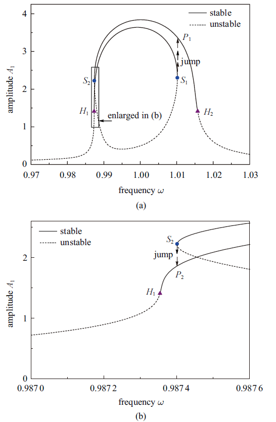
图1
含外激励van der Pol-Mathieu方程周期响应的频率响应曲线, $\omega$-$A_1$ 其中 $k_1=0.01$, $k_2=0.01$, $k_3=0.05$和$f=0.01$, (b)为(a)中标示区域的放大图
Fig.1
Frequency response curve $\omega$-$A_1$ of periodic response of the van der Pol-Mathieu equation with external excitation with $k_1=0.01$, $k_2=0.01$, $k_3=0.05$, and $f=0.01$, (b) is an enlarged view of a zone highlighted in (a)
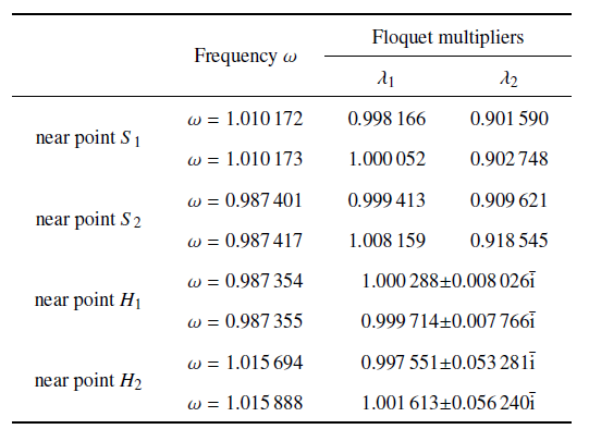
Table 1 Floquet multipliers $\lambda_1$ and $\lambda_2$ for the frequency $\omega$ near the four bifurcation points $S_1$, $S_2$, $H_1$, and $H_2$, where $\bar{\rm i}=\sqrt{-1}$
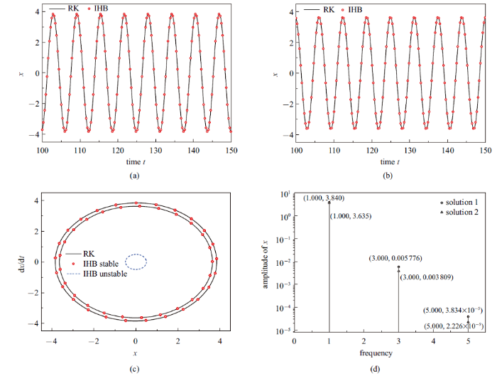
Fig.2
Three different periodic solutions of the van der Pol-Mathieu equation with external excitation for $\omega=1.0$ with $k_1=0.01$, $k_2=0.01$, $k_3=0.05$, and $f=0.01$: (a) Time history of the first stable periodic response; (b) time history of the second stable periodic response; (c) phase plane portraits of the three solutions; (d) Fourier spectra of the two stable periodic response
2 含外激励van der Pol-Mathieu方程的准周期运动
对于含外激励van der Pol-Mathieu方程的周期响应, 其频率成份之间是可约的, 例如在本文中, 系统的频率成份为$\omega$, $3\omega$和$5\omega$. 在上节分析得知, 系统的周期解经Hopf分岔后会产生准周期运动. 对准周期运动来说, 其频率成份至少含有两个或以上的不可约频率. 事实上, 本文首次发现了van der Pol-Mathieu方程的准周期运动的新特性, 即其频率成份是由落在$\omega$, $3\omega$和$5\omega$附近的边频带组成, 并且这些边频带里的频率是等相距的, 即为均匀的边频带. 此准周期运动的新特性, 正是由于van der Pol-Mathieu方程中的自激振动和参数激振相互作用产生的. 如若只考察van der Pol方程中的自激振动或只考察Mathieu方程的参数激振, 并不会产生准周期运动. 根据此准周期运动的新特性, 其频谱中含有两个基频, 一个是已知的频率$\omega$, 另一个可把它看作是均匀边频带里相邻频率的距离$\omega_{\rm d}$, 且$\omega_{\rm d}$事先是未知的, 此时准周期运动中所有的频率都可由这两个基频线性组合而成. 根据此特性, 发展了传统的IHB法, 引入两个时间尺度, 使之适用于精确求解含外激励van der Pol-Mathieu方程的准周期运动, 并且可以得到此准周期运动所有的频率成份.
2.1 两时间尺度的IHB法
相较于传统的IHB法, 两时间尺度的IHB法在求解含外激励van der Pol-Mathieu方程的准周期运动过程中有3点改进之处, 具体推导如下.
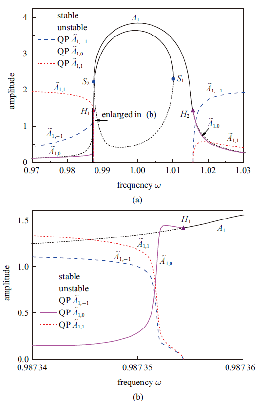
Fig.3
Frequency response curves $\omega$ -$A_1$ of periodic response and $\omega$ -$\tilde{A}_{1,-1}$, $\omega$ -$\tilde{A}_{1,0}$, and $\omega$ -$\tilde{A}_{1,1}$ of quasi-periodic (QP) motion of the van der Pol-Mathieu equation with external excitation with $k_1=0.01$, $k_2=0.01$, $k_3=0.05$, and $f=0.01$, (b) is an enlarged view of a zone highlighted in (a)
图4
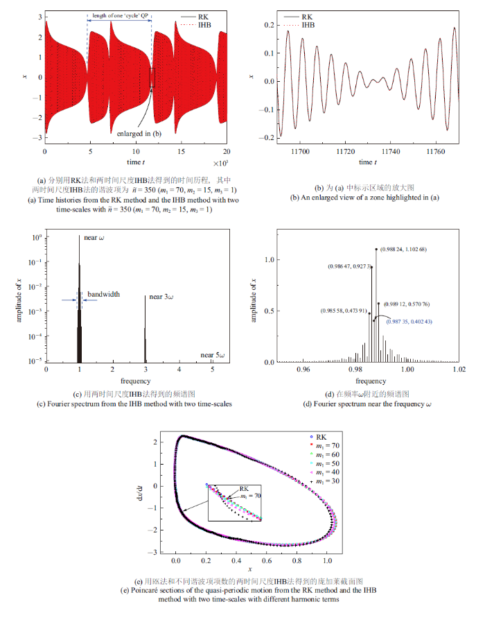
在分岔点$H_1$附近频率$\omega=0.987 35$时含外激励van der Pol-Mathieu方程的准周期运动, 其中 $k_1=0.01$, $k_2=0.01$, $k_3=0.05$和$f=0.01$
Fig.4
Quasi-periodic motion of the van der Pol-Mathieu equation with external excitation with $k_1=0.01$, $k_2=0.01$, $k_3=0.05$, and $f=0.01$ at the freqeuncy $\omega=0.987 35$ near the bifurcation point $H_1$
图5
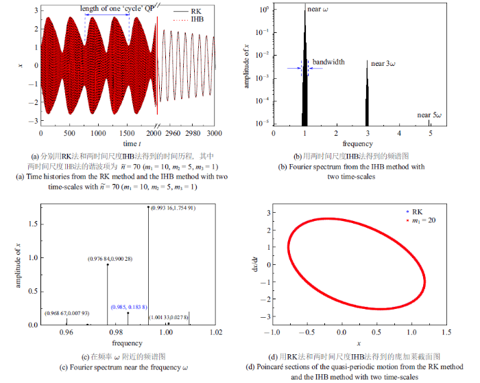
频率$\omega=0.985$时含外激励van der Pol-Mathieu方程的准周期运动, 其中 $k_1=0.01$, $k_2=0.01$, $k_3=0.05$和$f=0.01$
Fig.5
Quasi-periodic motion of the van der Pol-Mathieu equation with external excitation with $k_1=0.01$, $k_2=0.01$, $k_3=0.05$, and $f=0.01$ at the parametric excitation freqeuncy $\omega=0.985$
图6
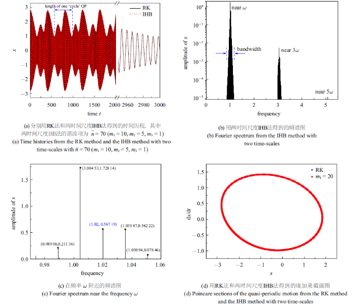
频率$\omega=1.020$时含外激励van der Pol-Mathieu方程的准周期运动, 其中 $k_1=0.01$, $k_2=0.01$, $k_3=0.05$和$f=0.01$
Fig.6
Quasi-periodic motion of the van der Pol-Mathieu equation with external excitation with $k_1=0.01$, $k_2=0.01$, $k_3=0.05$, and $f=0.01$ at the freqeuncy $\omega=1.020$}
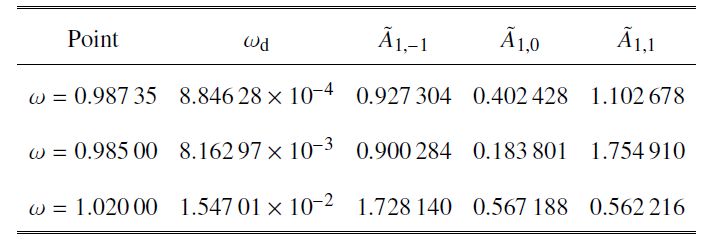
Table 2 A prior unknown $\omega_{\rm d}$ and three amplitudes $\tilde{A}_{1,-1}$, $\tilde{A}_{1,0}$, and $\tilde{A}_{1,1}$ in frequency response curves of the van der Pol-Mathieu equation with external excitation that are calculated by the IHB method with two time-scales at the three points $\omega=0.987 35,0.985,1.02$ in Fig.3
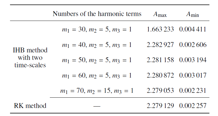
Table 3 Comparison of $A_{\text{max}}$ and $A_{\text{min}}$ from the RK method and the IHB method with two time-scales with different harmonic terms at the point $\omega=0.987 35$, where $A_{\text{max}}$ and $A_{\text{min}}$ are the maximal and minimal value of envelops of the quasi-periodic motions, respectively
An incremental harmonic balance method with two timescales for quasiperiodic motion of nonlinear systems whose spectrum contains uniformly spaced sideband frequencies
A new incremental harmonic balance method with two time scales for quasi-periodic motions of an axially moving beam with internal resonance under single-tone external excitation
Journal of Vibration and Acoustics, 2017,139(2):021010
HuangJL, ZhouWJ, ZhuWD.
Quasi-periodic motions of high-dimensional nonlinear models of a translating beam with a stationary load subsystem under harmonic boundary excitation
Transverse vibration of a rotor system driven by a cardan joint
1
1984
... 在工程中存在着很多可以用自激振动和参数激振联合作用的van der Pol-Mathieu方程来描述的振动, 例如, 含有万向接头的转子系统的横向振动[1], 卡盘作业过程中的参数激振[2], 含有自振和参数激振的齿轮装置系统的振动[3], 尘埃等离子体中的颗粒电荷的动力学行为[4], 高层建筑结构在风荷载下的振动[5-6]等, 都是可用van der Pol-Mathieu方程来描述振动的典型例子. van der Pol-Mathieu方程同时含有自激振动和参数激振, 蕴含着丰富的动力学行为, 多年来一直是众多学者关注点之一. ...
A study on parametric vibration in chuck work
1
1985
... 在工程中存在着很多可以用自激振动和参数激振联合作用的van der Pol-Mathieu方程来描述的振动, 例如, 含有万向接头的转子系统的横向振动[1], 卡盘作业过程中的参数激振[2], 含有自振和参数激振的齿轮装置系统的振动[3], 尘埃等离子体中的颗粒电荷的动力学行为[4], 高层建筑结构在风荷载下的振动[5-6]等, 都是可用van der Pol-Mathieu方程来描述振动的典型例子. van der Pol-Mathieu方程同时含有自激振动和参数激振, 蕴含着丰富的动力学行为, 多年来一直是众多学者关注点之一. ...
Synchronisation and chaos in a parametrically and self-excited system with two degrees of freedom
3
2000
... 在工程中存在着很多可以用自激振动和参数激振联合作用的van der Pol-Mathieu方程来描述的振动, 例如, 含有万向接头的转子系统的横向振动[1], 卡盘作业过程中的参数激振[2], 含有自振和参数激振的齿轮装置系统的振动[3], 尘埃等离子体中的颗粒电荷的动力学行为[4], 高层建筑结构在风荷载下的振动[5-6]等, 都是可用van der Pol-Mathieu方程来描述振动的典型例子. van der Pol-Mathieu方程同时含有自激振动和参数激振, 蕴含着丰富的动力学行为, 多年来一直是众多学者关注点之一. ...
... Tondl[7]首先分析了van der Pol-Mathieu方程中自激振动和参数激振的相互作用, 并在共振区域发现了周期响应. Kotera和Yano[8]用两个频率的和分析了van der Pol-Mathieu方程在参数共振区域的近似一阶和二阶的周期解. 陈予恕和徐鉴[9]研究了van der Pol-Duffing-Mathieu型系统主参数共振分岔解, 得到该非线性参数激励系统依赖于物理参数变化的振动模式. Szabelski和Warminski[10]分析了自激振动和参数激励对van der Pol-Mathieu方程的影响, 并且研究了附加外激励在同步区域内动力学行为的影响. Warminski等[3]对含有自激振动和参数激励的两自由度系统进行分析, 并得到了不同类型的响应, 包含有周期响应, 准周期运动响应和混沌. 彭献和陈自力[11]引入参数变换, 将强非线性系统转化为弱非线性系统, 利用摄动思想分析得到了van der Pol-Mathieu方程的1/2亚谐共振周期解. Belhaq和Fahsi[12]和Pandey等[13]分析了van der Pol-Mathieu-Duffing系统的响应, 得到该类系统可含有1:1锁频, 2:1次谐波锁频和准周期运动响应. 张琪昌等[14]利用改进的类Padé方法计算了van der Pol-Duffing方程的同异宿轨道. Warminski[15]研究了含有van der Pol和Rayleigh函数在两个不同自激振动模型下具有时滞状态的自激振动, 参数激振和强迫振动作用下的相互作用. 许多学者也对各类含有参数激振的非线性系统进行研究[16-19], 得到了不同的非线性振动特性和运动分岔. ...
... 早期对于van der Pol-Mathieu方程的众多研究主要集中在含有一个基频的周期响应及其稳定性分析. 可以利用不同的摄动方法求得这类方程的近似解析解[20]. 然而, 对于van der Pol-Mathieu方程来说, 因有自激振动与参数激励振动的相互耦合作用, 使得系统不仅有周期响应, 而且还有准周期运动响应, 甚至产生混沌, 近年来受到众多学者的关注. Belhaq和Houssni[21]为了构造准周期运动的近似解, 提出了双摄动的思想, 其方法包含了两个步骤: 第一步利用广义的平均法将准周期系统变为周期减化系统; 第二步是用多尺度法对周期减化系统构造出近似的准周期运动解. 他们利用双摄动方法得到了同时含有二次和三次非线性项的参数激励和外激励的单自由度系统的准周期解. 该双摄动方法的本质就是对周期减化系统在平衡点附近的周期解进行非线性近似, 该方法可进一步推广到各类非线性系统的准周期运动分析中[5-6,12,22]. Fan等[23]也利用了双摄动方法分析了van der Pol-Mathieu方程在有外激励和无外激励两种情况下的周期解和准周期运动近似解的包络线. 然而, 双摄动方法只能得到准周期运动包络线的最大和最小幅值, 无法得到系统准周期运动的具体响应情况, 更无法得到系统准周期运动的各个响应频率. Warminski等[3]和Warminski[15]利用多尺度法分别分析了含有自激励和参数激励的两个自由度时滞系统, 并利用数值法得到了两个时滞系统的准周期运动响应和混沌. Veerman和Verhulst[24]利用平均法分析了van der Pol-Mathieu方程, 并得到了由1阶和1/$\varepsilon$阶基础周期构造而成的准周期运动响应, 其中$\varepsilon$是小量. 上述的各种摄动法只能得到van der Pol-Mathieu方程准周期运动近似解, 有些方法得到的结果只能描述准周期运动的最大和最小振幅, 特别是在邻近分岔点处用摄动法得到的准周期运动解与数值解相差甚大, 据作者所知, 迄今为止尚未有有效的摄动法能精确地计算并得到此类van der Pol-Mathieu方程的精确准周期运动解. ...
A van der Pol-Mathieu equation for the dynamics of dust grain charge in dusty plasmas,
1
2007
... 在工程中存在着很多可以用自激振动和参数激振联合作用的van der Pol-Mathieu方程来描述的振动, 例如, 含有万向接头的转子系统的横向振动[1], 卡盘作业过程中的参数激振[2], 含有自振和参数激振的齿轮装置系统的振动[3], 尘埃等离子体中的颗粒电荷的动力学行为[4], 高层建筑结构在风荷载下的振动[5-6]等, 都是可用van der Pol-Mathieu方程来描述振动的典型例子. van der Pol-Mathieu方程同时含有自激振动和参数激振, 蕴含着丰富的动力学行为, 多年来一直是众多学者关注点之一. ...
Periodic and quasiperiodic galloping of a wind-excited tower under external excitation
2
2013
... 在工程中存在着很多可以用自激振动和参数激振联合作用的van der Pol-Mathieu方程来描述的振动, 例如, 含有万向接头的转子系统的横向振动[1], 卡盘作业过程中的参数激振[2], 含有自振和参数激振的齿轮装置系统的振动[3], 尘埃等离子体中的颗粒电荷的动力学行为[4], 高层建筑结构在风荷载下的振动[5-6]等, 都是可用van der Pol-Mathieu方程来描述振动的典型例子. van der Pol-Mathieu方程同时含有自激振动和参数激振, 蕴含着丰富的动力学行为, 多年来一直是众多学者关注点之一. ...
... 早期对于van der Pol-Mathieu方程的众多研究主要集中在含有一个基频的周期响应及其稳定性分析. 可以利用不同的摄动方法求得这类方程的近似解析解[20]. 然而, 对于van der Pol-Mathieu方程来说, 因有自激振动与参数激励振动的相互耦合作用, 使得系统不仅有周期响应, 而且还有准周期运动响应, 甚至产生混沌, 近年来受到众多学者的关注. Belhaq和Houssni[21]为了构造准周期运动的近似解, 提出了双摄动的思想, 其方法包含了两个步骤: 第一步利用广义的平均法将准周期系统变为周期减化系统; 第二步是用多尺度法对周期减化系统构造出近似的准周期运动解. 他们利用双摄动方法得到了同时含有二次和三次非线性项的参数激励和外激励的单自由度系统的准周期解. 该双摄动方法的本质就是对周期减化系统在平衡点附近的周期解进行非线性近似, 该方法可进一步推广到各类非线性系统的准周期运动分析中[5-6,12,22]. Fan等[23]也利用了双摄动方法分析了van der Pol-Mathieu方程在有外激励和无外激励两种情况下的周期解和准周期运动近似解的包络线. 然而, 双摄动方法只能得到准周期运动包络线的最大和最小幅值, 无法得到系统准周期运动的具体响应情况, 更无法得到系统准周期运动的各个响应频率. Warminski等[3]和Warminski[15]利用多尺度法分别分析了含有自激励和参数激励的两个自由度时滞系统, 并利用数值法得到了两个时滞系统的准周期运动响应和混沌. Veerman和Verhulst[24]利用平均法分析了van der Pol-Mathieu方程, 并得到了由1阶和1/$\varepsilon$阶基础周期构造而成的准周期运动响应, 其中$\varepsilon$是小量. 上述的各种摄动法只能得到van der Pol-Mathieu方程准周期运动近似解, 有些方法得到的结果只能描述准周期运动的最大和最小振幅, 特别是在邻近分岔点处用摄动法得到的准周期运动解与数值解相差甚大, 据作者所知, 迄今为止尚未有有效的摄动法能精确地计算并得到此类van der Pol-Mathieu方程的精确准周期运动解. ...
On the quasiperiodic galloping of a wind-excited tower
2
2013
... 在工程中存在着很多可以用自激振动和参数激振联合作用的van der Pol-Mathieu方程来描述的振动, 例如, 含有万向接头的转子系统的横向振动[1], 卡盘作业过程中的参数激振[2], 含有自振和参数激振的齿轮装置系统的振动[3], 尘埃等离子体中的颗粒电荷的动力学行为[4], 高层建筑结构在风荷载下的振动[5-6]等, 都是可用van der Pol-Mathieu方程来描述振动的典型例子. van der Pol-Mathieu方程同时含有自激振动和参数激振, 蕴含着丰富的动力学行为, 多年来一直是众多学者关注点之一. ...
... 早期对于van der Pol-Mathieu方程的众多研究主要集中在含有一个基频的周期响应及其稳定性分析. 可以利用不同的摄动方法求得这类方程的近似解析解[20]. 然而, 对于van der Pol-Mathieu方程来说, 因有自激振动与参数激励振动的相互耦合作用, 使得系统不仅有周期响应, 而且还有准周期运动响应, 甚至产生混沌, 近年来受到众多学者的关注. Belhaq和Houssni[21]为了构造准周期运动的近似解, 提出了双摄动的思想, 其方法包含了两个步骤: 第一步利用广义的平均法将准周期系统变为周期减化系统; 第二步是用多尺度法对周期减化系统构造出近似的准周期运动解. 他们利用双摄动方法得到了同时含有二次和三次非线性项的参数激励和外激励的单自由度系统的准周期解. 该双摄动方法的本质就是对周期减化系统在平衡点附近的周期解进行非线性近似, 该方法可进一步推广到各类非线性系统的准周期运动分析中[5-6,12,22]. Fan等[23]也利用了双摄动方法分析了van der Pol-Mathieu方程在有外激励和无外激励两种情况下的周期解和准周期运动近似解的包络线. 然而, 双摄动方法只能得到准周期运动包络线的最大和最小幅值, 无法得到系统准周期运动的具体响应情况, 更无法得到系统准周期运动的各个响应频率. Warminski等[3]和Warminski[15]利用多尺度法分别分析了含有自激励和参数激励的两个自由度时滞系统, 并利用数值法得到了两个时滞系统的准周期运动响应和混沌. Veerman和Verhulst[24]利用平均法分析了van der Pol-Mathieu方程, 并得到了由1阶和1/$\varepsilon$阶基础周期构造而成的准周期运动响应, 其中$\varepsilon$是小量. 上述的各种摄动法只能得到van der Pol-Mathieu方程准周期运动近似解, 有些方法得到的结果只能描述准周期运动的最大和最小振幅, 特别是在邻近分岔点处用摄动法得到的准周期运动解与数值解相差甚大, 据作者所知, 迄今为止尚未有有效的摄动法能精确地计算并得到此类van der Pol-Mathieu方程的精确准周期运动解. ...
On the interaction between self-excited and parametric vibrations. National Research Institute for Machine Design, Monographs and Memoranda No. 25,
1
1978
... Tondl[7]首先分析了van der Pol-Mathieu方程中自激振动和参数激振的相互作用, 并在共振区域发现了周期响应. Kotera和Yano[8]用两个频率的和分析了van der Pol-Mathieu方程在参数共振区域的近似一阶和二阶的周期解. 陈予恕和徐鉴[9]研究了van der Pol-Duffing-Mathieu型系统主参数共振分岔解, 得到该非线性参数激励系统依赖于物理参数变化的振动模式. Szabelski和Warminski[10]分析了自激振动和参数激励对van der Pol-Mathieu方程的影响, 并且研究了附加外激励在同步区域内动力学行为的影响. Warminski等[3]对含有自激振动和参数激励的两自由度系统进行分析, 并得到了不同类型的响应, 包含有周期响应, 准周期运动响应和混沌. 彭献和陈自力[11]引入参数变换, 将强非线性系统转化为弱非线性系统, 利用摄动思想分析得到了van der Pol-Mathieu方程的1/2亚谐共振周期解. Belhaq和Fahsi[12]和Pandey等[13]分析了van der Pol-Mathieu-Duffing系统的响应, 得到该类系统可含有1:1锁频, 2:1次谐波锁频和准周期运动响应. 张琪昌等[14]利用改进的类Padé方法计算了van der Pol-Duffing方程的同异宿轨道. Warminski[15]研究了含有van der Pol和Rayleigh函数在两个不同自激振动模型下具有时滞状态的自激振动, 参数激振和强迫振动作用下的相互作用. 许多学者也对各类含有参数激振的非线性系统进行研究[16-19], 得到了不同的非线性振动特性和运动分岔. ...
Periodic solutions and the stability in a non-linear parametric excitation system
1
1985
... Tondl[7]首先分析了van der Pol-Mathieu方程中自激振动和参数激振的相互作用, 并在共振区域发现了周期响应. Kotera和Yano[8]用两个频率的和分析了van der Pol-Mathieu方程在参数共振区域的近似一阶和二阶的周期解. 陈予恕和徐鉴[9]研究了van der Pol-Duffing-Mathieu型系统主参数共振分岔解, 得到该非线性参数激励系统依赖于物理参数变化的振动模式. Szabelski和Warminski[10]分析了自激振动和参数激励对van der Pol-Mathieu方程的影响, 并且研究了附加外激励在同步区域内动力学行为的影响. Warminski等[3]对含有自激振动和参数激励的两自由度系统进行分析, 并得到了不同类型的响应, 包含有周期响应, 准周期运动响应和混沌. 彭献和陈自力[11]引入参数变换, 将强非线性系统转化为弱非线性系统, 利用摄动思想分析得到了van der Pol-Mathieu方程的1/2亚谐共振周期解. Belhaq和Fahsi[12]和Pandey等[13]分析了van der Pol-Mathieu-Duffing系统的响应, 得到该类系统可含有1:1锁频, 2:1次谐波锁频和准周期运动响应. 张琪昌等[14]利用改进的类Padé方法计算了van der Pol-Duffing方程的同异宿轨道. Warminski[15]研究了含有van der Pol和Rayleigh函数在两个不同自激振动模型下具有时滞状态的自激振动, 参数激振和强迫振动作用下的相互作用. 许多学者也对各类含有参数激振的非线性系统进行研究[16-19], 得到了不同的非线性振动特性和运动分岔. ...
Van der pol-Duffing-Mathieu型系统主参数共振分岔解的普适分类
1
1995
... Tondl[7]首先分析了van der Pol-Mathieu方程中自激振动和参数激振的相互作用, 并在共振区域发现了周期响应. Kotera和Yano[8]用两个频率的和分析了van der Pol-Mathieu方程在参数共振区域的近似一阶和二阶的周期解. 陈予恕和徐鉴[9]研究了van der Pol-Duffing-Mathieu型系统主参数共振分岔解, 得到该非线性参数激励系统依赖于物理参数变化的振动模式. Szabelski和Warminski[10]分析了自激振动和参数激励对van der Pol-Mathieu方程的影响, 并且研究了附加外激励在同步区域内动力学行为的影响. Warminski等[3]对含有自激振动和参数激励的两自由度系统进行分析, 并得到了不同类型的响应, 包含有周期响应, 准周期运动响应和混沌. 彭献和陈自力[11]引入参数变换, 将强非线性系统转化为弱非线性系统, 利用摄动思想分析得到了van der Pol-Mathieu方程的1/2亚谐共振周期解. Belhaq和Fahsi[12]和Pandey等[13]分析了van der Pol-Mathieu-Duffing系统的响应, 得到该类系统可含有1:1锁频, 2:1次谐波锁频和准周期运动响应. 张琪昌等[14]利用改进的类Padé方法计算了van der Pol-Duffing方程的同异宿轨道. Warminski[15]研究了含有van der Pol和Rayleigh函数在两个不同自激振动模型下具有时滞状态的自激振动, 参数激振和强迫振动作用下的相互作用. 许多学者也对各类含有参数激振的非线性系统进行研究[16-19], 得到了不同的非线性振动特性和运动分岔. ...
Self-excited system vibrations with parametric and external excitation
1
1995
... Tondl[7]首先分析了van der Pol-Mathieu方程中自激振动和参数激振的相互作用, 并在共振区域发现了周期响应. Kotera和Yano[8]用两个频率的和分析了van der Pol-Mathieu方程在参数共振区域的近似一阶和二阶的周期解. 陈予恕和徐鉴[9]研究了van der Pol-Duffing-Mathieu型系统主参数共振分岔解, 得到该非线性参数激励系统依赖于物理参数变化的振动模式. Szabelski和Warminski[10]分析了自激振动和参数激励对van der Pol-Mathieu方程的影响, 并且研究了附加外激励在同步区域内动力学行为的影响. Warminski等[3]对含有自激振动和参数激励的两自由度系统进行分析, 并得到了不同类型的响应, 包含有周期响应, 准周期运动响应和混沌. 彭献和陈自力[11]引入参数变换, 将强非线性系统转化为弱非线性系统, 利用摄动思想分析得到了van der Pol-Mathieu方程的1/2亚谐共振周期解. Belhaq和Fahsi[12]和Pandey等[13]分析了van der Pol-Mathieu-Duffing系统的响应, 得到该类系统可含有1:1锁频, 2:1次谐波锁频和准周期运动响应. 张琪昌等[14]利用改进的类Padé方法计算了van der Pol-Duffing方程的同异宿轨道. Warminski[15]研究了含有van der Pol和Rayleigh函数在两个不同自激振动模型下具有时滞状态的自激振动, 参数激振和强迫振动作用下的相互作用. 许多学者也对各类含有参数激振的非线性系统进行研究[16-19], 得到了不同的非线性振动特性和运动分岔. ...
一类强非线性系统共振周期解的渐近分析
1
2004
... Tondl[7]首先分析了van der Pol-Mathieu方程中自激振动和参数激振的相互作用, 并在共振区域发现了周期响应. Kotera和Yano[8]用两个频率的和分析了van der Pol-Mathieu方程在参数共振区域的近似一阶和二阶的周期解. 陈予恕和徐鉴[9]研究了van der Pol-Duffing-Mathieu型系统主参数共振分岔解, 得到该非线性参数激励系统依赖于物理参数变化的振动模式. Szabelski和Warminski[10]分析了自激振动和参数激励对van der Pol-Mathieu方程的影响, 并且研究了附加外激励在同步区域内动力学行为的影响. Warminski等[3]对含有自激振动和参数激励的两自由度系统进行分析, 并得到了不同类型的响应, 包含有周期响应, 准周期运动响应和混沌. 彭献和陈自力[11]引入参数变换, 将强非线性系统转化为弱非线性系统, 利用摄动思想分析得到了van der Pol-Mathieu方程的1/2亚谐共振周期解. Belhaq和Fahsi[12]和Pandey等[13]分析了van der Pol-Mathieu-Duffing系统的响应, 得到该类系统可含有1:1锁频, 2:1次谐波锁频和准周期运动响应. 张琪昌等[14]利用改进的类Padé方法计算了van der Pol-Duffing方程的同异宿轨道. Warminski[15]研究了含有van der Pol和Rayleigh函数在两个不同自激振动模型下具有时滞状态的自激振动, 参数激振和强迫振动作用下的相互作用. 许多学者也对各类含有参数激振的非线性系统进行研究[16-19], 得到了不同的非线性振动特性和运动分岔. ...
2:1 and 1:1 frequency-locking in fast excited van der Pol-Mathieu-Duffing oscillator
2
2007
... Tondl[7]首先分析了van der Pol-Mathieu方程中自激振动和参数激振的相互作用, 并在共振区域发现了周期响应. Kotera和Yano[8]用两个频率的和分析了van der Pol-Mathieu方程在参数共振区域的近似一阶和二阶的周期解. 陈予恕和徐鉴[9]研究了van der Pol-Duffing-Mathieu型系统主参数共振分岔解, 得到该非线性参数激励系统依赖于物理参数变化的振动模式. Szabelski和Warminski[10]分析了自激振动和参数激励对van der Pol-Mathieu方程的影响, 并且研究了附加外激励在同步区域内动力学行为的影响. Warminski等[3]对含有自激振动和参数激励的两自由度系统进行分析, 并得到了不同类型的响应, 包含有周期响应, 准周期运动响应和混沌. 彭献和陈自力[11]引入参数变换, 将强非线性系统转化为弱非线性系统, 利用摄动思想分析得到了van der Pol-Mathieu方程的1/2亚谐共振周期解. Belhaq和Fahsi[12]和Pandey等[13]分析了van der Pol-Mathieu-Duffing系统的响应, 得到该类系统可含有1:1锁频, 2:1次谐波锁频和准周期运动响应. 张琪昌等[14]利用改进的类Padé方法计算了van der Pol-Duffing方程的同异宿轨道. Warminski[15]研究了含有van der Pol和Rayleigh函数在两个不同自激振动模型下具有时滞状态的自激振动, 参数激振和强迫振动作用下的相互作用. 许多学者也对各类含有参数激振的非线性系统进行研究[16-19], 得到了不同的非线性振动特性和运动分岔. ...
... 早期对于van der Pol-Mathieu方程的众多研究主要集中在含有一个基频的周期响应及其稳定性分析. 可以利用不同的摄动方法求得这类方程的近似解析解[20]. 然而, 对于van der Pol-Mathieu方程来说, 因有自激振动与参数激励振动的相互耦合作用, 使得系统不仅有周期响应, 而且还有准周期运动响应, 甚至产生混沌, 近年来受到众多学者的关注. Belhaq和Houssni[21]为了构造准周期运动的近似解, 提出了双摄动的思想, 其方法包含了两个步骤: 第一步利用广义的平均法将准周期系统变为周期减化系统; 第二步是用多尺度法对周期减化系统构造出近似的准周期运动解. 他们利用双摄动方法得到了同时含有二次和三次非线性项的参数激励和外激励的单自由度系统的准周期解. 该双摄动方法的本质就是对周期减化系统在平衡点附近的周期解进行非线性近似, 该方法可进一步推广到各类非线性系统的准周期运动分析中[5-6,12,22]. Fan等[23]也利用了双摄动方法分析了van der Pol-Mathieu方程在有外激励和无外激励两种情况下的周期解和准周期运动近似解的包络线. 然而, 双摄动方法只能得到准周期运动包络线的最大和最小幅值, 无法得到系统准周期运动的具体响应情况, 更无法得到系统准周期运动的各个响应频率. Warminski等[3]和Warminski[15]利用多尺度法分别分析了含有自激励和参数激励的两个自由度时滞系统, 并利用数值法得到了两个时滞系统的准周期运动响应和混沌. Veerman和Verhulst[24]利用平均法分析了van der Pol-Mathieu方程, 并得到了由1阶和1/$\varepsilon$阶基础周期构造而成的准周期运动响应, 其中$\varepsilon$是小量. 上述的各种摄动法只能得到van der Pol-Mathieu方程准周期运动近似解, 有些方法得到的结果只能描述准周期运动的最大和最小振幅, 特别是在邻近分岔点处用摄动法得到的准周期运动解与数值解相差甚大, 据作者所知, 迄今为止尚未有有效的摄动法能精确地计算并得到此类van der Pol-Mathieu方程的精确准周期运动解. ...
Frequency locking in a forced Mathieu-van der Pol-Duffing system
1
2007
... Tondl[7]首先分析了van der Pol-Mathieu方程中自激振动和参数激振的相互作用, 并在共振区域发现了周期响应. Kotera和Yano[8]用两个频率的和分析了van der Pol-Mathieu方程在参数共振区域的近似一阶和二阶的周期解. 陈予恕和徐鉴[9]研究了van der Pol-Duffing-Mathieu型系统主参数共振分岔解, 得到该非线性参数激励系统依赖于物理参数变化的振动模式. Szabelski和Warminski[10]分析了自激振动和参数激励对van der Pol-Mathieu方程的影响, 并且研究了附加外激励在同步区域内动力学行为的影响. Warminski等[3]对含有自激振动和参数激励的两自由度系统进行分析, 并得到了不同类型的响应, 包含有周期响应, 准周期运动响应和混沌. 彭献和陈自力[11]引入参数变换, 将强非线性系统转化为弱非线性系统, 利用摄动思想分析得到了van der Pol-Mathieu方程的1/2亚谐共振周期解. Belhaq和Fahsi[12]和Pandey等[13]分析了van der Pol-Mathieu-Duffing系统的响应, 得到该类系统可含有1:1锁频, 2:1次谐波锁频和准周期运动响应. 张琪昌等[14]利用改进的类Padé方法计算了van der Pol-Duffing方程的同异宿轨道. Warminski[15]研究了含有van der Pol和Rayleigh函数在两个不同自激振动模型下具有时滞状态的自激振动, 参数激振和强迫振动作用下的相互作用. 许多学者也对各类含有参数激振的非线性系统进行研究[16-19], 得到了不同的非线性振动特性和运动分岔. ...
类Padé逼近方法在二维非线性振动系统的应用
1
2011
... Tondl[7]首先分析了van der Pol-Mathieu方程中自激振动和参数激振的相互作用, 并在共振区域发现了周期响应. Kotera和Yano[8]用两个频率的和分析了van der Pol-Mathieu方程在参数共振区域的近似一阶和二阶的周期解. 陈予恕和徐鉴[9]研究了van der Pol-Duffing-Mathieu型系统主参数共振分岔解, 得到该非线性参数激励系统依赖于物理参数变化的振动模式. Szabelski和Warminski[10]分析了自激振动和参数激励对van der Pol-Mathieu方程的影响, 并且研究了附加外激励在同步区域内动力学行为的影响. Warminski等[3]对含有自激振动和参数激励的两自由度系统进行分析, 并得到了不同类型的响应, 包含有周期响应, 准周期运动响应和混沌. 彭献和陈自力[11]引入参数变换, 将强非线性系统转化为弱非线性系统, 利用摄动思想分析得到了van der Pol-Mathieu方程的1/2亚谐共振周期解. Belhaq和Fahsi[12]和Pandey等[13]分析了van der Pol-Mathieu-Duffing系统的响应, 得到该类系统可含有1:1锁频, 2:1次谐波锁频和准周期运动响应. 张琪昌等[14]利用改进的类Padé方法计算了van der Pol-Duffing方程的同异宿轨道. Warminski[15]研究了含有van der Pol和Rayleigh函数在两个不同自激振动模型下具有时滞状态的自激振动, 参数激振和强迫振动作用下的相互作用. 许多学者也对各类含有参数激振的非线性系统进行研究[16-19], 得到了不同的非线性振动特性和运动分岔. ...
Nonlinear dynamics of self-, parametric, and externally excited oscillator with time delay: van der Pol versus Rayleigh models
2
2019
... Tondl[7]首先分析了van der Pol-Mathieu方程中自激振动和参数激振的相互作用, 并在共振区域发现了周期响应. Kotera和Yano[8]用两个频率的和分析了van der Pol-Mathieu方程在参数共振区域的近似一阶和二阶的周期解. 陈予恕和徐鉴[9]研究了van der Pol-Duffing-Mathieu型系统主参数共振分岔解, 得到该非线性参数激励系统依赖于物理参数变化的振动模式. Szabelski和Warminski[10]分析了自激振动和参数激励对van der Pol-Mathieu方程的影响, 并且研究了附加外激励在同步区域内动力学行为的影响. Warminski等[3]对含有自激振动和参数激励的两自由度系统进行分析, 并得到了不同类型的响应, 包含有周期响应, 准周期运动响应和混沌. 彭献和陈自力[11]引入参数变换, 将强非线性系统转化为弱非线性系统, 利用摄动思想分析得到了van der Pol-Mathieu方程的1/2亚谐共振周期解. Belhaq和Fahsi[12]和Pandey等[13]分析了van der Pol-Mathieu-Duffing系统的响应, 得到该类系统可含有1:1锁频, 2:1次谐波锁频和准周期运动响应. 张琪昌等[14]利用改进的类Padé方法计算了van der Pol-Duffing方程的同异宿轨道. Warminski[15]研究了含有van der Pol和Rayleigh函数在两个不同自激振动模型下具有时滞状态的自激振动, 参数激振和强迫振动作用下的相互作用. 许多学者也对各类含有参数激振的非线性系统进行研究[16-19], 得到了不同的非线性振动特性和运动分岔. ...
... 早期对于van der Pol-Mathieu方程的众多研究主要集中在含有一个基频的周期响应及其稳定性分析. 可以利用不同的摄动方法求得这类方程的近似解析解[20]. 然而, 对于van der Pol-Mathieu方程来说, 因有自激振动与参数激励振动的相互耦合作用, 使得系统不仅有周期响应, 而且还有准周期运动响应, 甚至产生混沌, 近年来受到众多学者的关注. Belhaq和Houssni[21]为了构造准周期运动的近似解, 提出了双摄动的思想, 其方法包含了两个步骤: 第一步利用广义的平均法将准周期系统变为周期减化系统; 第二步是用多尺度法对周期减化系统构造出近似的准周期运动解. 他们利用双摄动方法得到了同时含有二次和三次非线性项的参数激励和外激励的单自由度系统的准周期解. 该双摄动方法的本质就是对周期减化系统在平衡点附近的周期解进行非线性近似, 该方法可进一步推广到各类非线性系统的准周期运动分析中[5-6,12,22]. Fan等[23]也利用了双摄动方法分析了van der Pol-Mathieu方程在有外激励和无外激励两种情况下的周期解和准周期运动近似解的包络线. 然而, 双摄动方法只能得到准周期运动包络线的最大和最小幅值, 无法得到系统准周期运动的具体响应情况, 更无法得到系统准周期运动的各个响应频率. Warminski等[3]和Warminski[15]利用多尺度法分别分析了含有自激励和参数激励的两个自由度时滞系统, 并利用数值法得到了两个时滞系统的准周期运动响应和混沌. Veerman和Verhulst[24]利用平均法分析了van der Pol-Mathieu方程, 并得到了由1阶和1/$\varepsilon$阶基础周期构造而成的准周期运动响应, 其中$\varepsilon$是小量. 上述的各种摄动法只能得到van der Pol-Mathieu方程准周期运动近似解, 有些方法得到的结果只能描述准周期运动的最大和最小振幅, 特别是在邻近分岔点处用摄动法得到的准周期运动解与数值解相差甚大, 据作者所知, 迄今为止尚未有有效的摄动法能精确地计算并得到此类van der Pol-Mathieu方程的精确准周期运动解. ...
凸肩叶片的非线性振动特性与运动分岔
1
2011
... Tondl[7]首先分析了van der Pol-Mathieu方程中自激振动和参数激振的相互作用, 并在共振区域发现了周期响应. Kotera和Yano[8]用两个频率的和分析了van der Pol-Mathieu方程在参数共振区域的近似一阶和二阶的周期解. 陈予恕和徐鉴[9]研究了van der Pol-Duffing-Mathieu型系统主参数共振分岔解, 得到该非线性参数激励系统依赖于物理参数变化的振动模式. Szabelski和Warminski[10]分析了自激振动和参数激励对van der Pol-Mathieu方程的影响, 并且研究了附加外激励在同步区域内动力学行为的影响. Warminski等[3]对含有自激振动和参数激励的两自由度系统进行分析, 并得到了不同类型的响应, 包含有周期响应, 准周期运动响应和混沌. 彭献和陈自力[11]引入参数变换, 将强非线性系统转化为弱非线性系统, 利用摄动思想分析得到了van der Pol-Mathieu方程的1/2亚谐共振周期解. Belhaq和Fahsi[12]和Pandey等[13]分析了van der Pol-Mathieu-Duffing系统的响应, 得到该类系统可含有1:1锁频, 2:1次谐波锁频和准周期运动响应. 张琪昌等[14]利用改进的类Padé方法计算了van der Pol-Duffing方程的同异宿轨道. Warminski[15]研究了含有van der Pol和Rayleigh函数在两个不同自激振动模型下具有时滞状态的自激振动, 参数激振和强迫振动作用下的相互作用. 许多学者也对各类含有参数激振的非线性系统进行研究[16-19], 得到了不同的非线性振动特性和运动分岔. ...
非齐次边界条件下轴向运动梁的非线性振动
0
2019
非齐次边界条件下轴向运动梁的非线性振动
0
2019
2:1 内共振条件下变转速预变形叶片的非线性动力学响应
0
2020
2:1 内共振条件下变转速预变形叶片的非线性动力学响应
0
2020
Duffing 型系统的不动点混沌和 Fold/Fold 簇发现象及机理分析
1
2020
... Tondl[7]首先分析了van der Pol-Mathieu方程中自激振动和参数激振的相互作用, 并在共振区域发现了周期响应. Kotera和Yano[8]用两个频率的和分析了van der Pol-Mathieu方程在参数共振区域的近似一阶和二阶的周期解. 陈予恕和徐鉴[9]研究了van der Pol-Duffing-Mathieu型系统主参数共振分岔解, 得到该非线性参数激励系统依赖于物理参数变化的振动模式. Szabelski和Warminski[10]分析了自激振动和参数激励对van der Pol-Mathieu方程的影响, 并且研究了附加外激励在同步区域内动力学行为的影响. Warminski等[3]对含有自激振动和参数激励的两自由度系统进行分析, 并得到了不同类型的响应, 包含有周期响应, 准周期运动响应和混沌. 彭献和陈自力[11]引入参数变换, 将强非线性系统转化为弱非线性系统, 利用摄动思想分析得到了van der Pol-Mathieu方程的1/2亚谐共振周期解. Belhaq和Fahsi[12]和Pandey等[13]分析了van der Pol-Mathieu-Duffing系统的响应, 得到该类系统可含有1:1锁频, 2:1次谐波锁频和准周期运动响应. 张琪昌等[14]利用改进的类Padé方法计算了van der Pol-Duffing方程的同异宿轨道. Warminski[15]研究了含有van der Pol和Rayleigh函数在两个不同自激振动模型下具有时滞状态的自激振动, 参数激振和强迫振动作用下的相互作用. 许多学者也对各类含有参数激振的非线性系统进行研究[16-19], 得到了不同的非线性振动特性和运动分岔. ...
Nonlinear Oscillations
1
1995
... 早期对于van der Pol-Mathieu方程的众多研究主要集中在含有一个基频的周期响应及其稳定性分析. 可以利用不同的摄动方法求得这类方程的近似解析解[20]. 然而, 对于van der Pol-Mathieu方程来说, 因有自激振动与参数激励振动的相互耦合作用, 使得系统不仅有周期响应, 而且还有准周期运动响应, 甚至产生混沌, 近年来受到众多学者的关注. Belhaq和Houssni[21]为了构造准周期运动的近似解, 提出了双摄动的思想, 其方法包含了两个步骤: 第一步利用广义的平均法将准周期系统变为周期减化系统; 第二步是用多尺度法对周期减化系统构造出近似的准周期运动解. 他们利用双摄动方法得到了同时含有二次和三次非线性项的参数激励和外激励的单自由度系统的准周期解. 该双摄动方法的本质就是对周期减化系统在平衡点附近的周期解进行非线性近似, 该方法可进一步推广到各类非线性系统的准周期运动分析中[5-6,12,22]. Fan等[23]也利用了双摄动方法分析了van der Pol-Mathieu方程在有外激励和无外激励两种情况下的周期解和准周期运动近似解的包络线. 然而, 双摄动方法只能得到准周期运动包络线的最大和最小幅值, 无法得到系统准周期运动的具体响应情况, 更无法得到系统准周期运动的各个响应频率. Warminski等[3]和Warminski[15]利用多尺度法分别分析了含有自激励和参数激励的两个自由度时滞系统, 并利用数值法得到了两个时滞系统的准周期运动响应和混沌. Veerman和Verhulst[24]利用平均法分析了van der Pol-Mathieu方程, 并得到了由1阶和1/$\varepsilon$阶基础周期构造而成的准周期运动响应, 其中$\varepsilon$是小量. 上述的各种摄动法只能得到van der Pol-Mathieu方程准周期运动近似解, 有些方法得到的结果只能描述准周期运动的最大和最小振幅, 特别是在邻近分岔点处用摄动法得到的准周期运动解与数值解相差甚大, 据作者所知, 迄今为止尚未有有效的摄动法能精确地计算并得到此类van der Pol-Mathieu方程的精确准周期运动解. ...
Quasi-periodic oscillations, chaos and suppression of chaos in a nonlinear oscillator driven by parametric and external excitations
1
1999
... 早期对于van der Pol-Mathieu方程的众多研究主要集中在含有一个基频的周期响应及其稳定性分析. 可以利用不同的摄动方法求得这类方程的近似解析解[20]. 然而, 对于van der Pol-Mathieu方程来说, 因有自激振动与参数激励振动的相互耦合作用, 使得系统不仅有周期响应, 而且还有准周期运动响应, 甚至产生混沌, 近年来受到众多学者的关注. Belhaq和Houssni[21]为了构造准周期运动的近似解, 提出了双摄动的思想, 其方法包含了两个步骤: 第一步利用广义的平均法将准周期系统变为周期减化系统; 第二步是用多尺度法对周期减化系统构造出近似的准周期运动解. 他们利用双摄动方法得到了同时含有二次和三次非线性项的参数激励和外激励的单自由度系统的准周期解. 该双摄动方法的本质就是对周期减化系统在平衡点附近的周期解进行非线性近似, 该方法可进一步推广到各类非线性系统的准周期运动分析中[5-6,12,22]. Fan等[23]也利用了双摄动方法分析了van der Pol-Mathieu方程在有外激励和无外激励两种情况下的周期解和准周期运动近似解的包络线. 然而, 双摄动方法只能得到准周期运动包络线的最大和最小幅值, 无法得到系统准周期运动的具体响应情况, 更无法得到系统准周期运动的各个响应频率. Warminski等[3]和Warminski[15]利用多尺度法分别分析了含有自激励和参数激励的两个自由度时滞系统, 并利用数值法得到了两个时滞系统的准周期运动响应和混沌. Veerman和Verhulst[24]利用平均法分析了van der Pol-Mathieu方程, 并得到了由1阶和1/$\varepsilon$阶基础周期构造而成的准周期运动响应, 其中$\varepsilon$是小量. 上述的各种摄动法只能得到van der Pol-Mathieu方程准周期运动近似解, 有些方法得到的结果只能描述准周期运动的最大和最小振幅, 特别是在邻近分岔点处用摄动法得到的准周期运动解与数值解相差甚大, 据作者所知, 迄今为止尚未有有效的摄动法能精确地计算并得到此类van der Pol-Mathieu方程的精确准周期运动解. ...
Three-period quasi-periodic solutions in the self-excited quasi-periodic Mathieu oscillator
1
2005
... 早期对于van der Pol-Mathieu方程的众多研究主要集中在含有一个基频的周期响应及其稳定性分析. 可以利用不同的摄动方法求得这类方程的近似解析解[20]. 然而, 对于van der Pol-Mathieu方程来说, 因有自激振动与参数激励振动的相互耦合作用, 使得系统不仅有周期响应, 而且还有准周期运动响应, 甚至产生混沌, 近年来受到众多学者的关注. Belhaq和Houssni[21]为了构造准周期运动的近似解, 提出了双摄动的思想, 其方法包含了两个步骤: 第一步利用广义的平均法将准周期系统变为周期减化系统; 第二步是用多尺度法对周期减化系统构造出近似的准周期运动解. 他们利用双摄动方法得到了同时含有二次和三次非线性项的参数激励和外激励的单自由度系统的准周期解. 该双摄动方法的本质就是对周期减化系统在平衡点附近的周期解进行非线性近似, 该方法可进一步推广到各类非线性系统的准周期运动分析中[5-6,12,22]. Fan等[23]也利用了双摄动方法分析了van der Pol-Mathieu方程在有外激励和无外激励两种情况下的周期解和准周期运动近似解的包络线. 然而, 双摄动方法只能得到准周期运动包络线的最大和最小幅值, 无法得到系统准周期运动的具体响应情况, 更无法得到系统准周期运动的各个响应频率. Warminski等[3]和Warminski[15]利用多尺度法分别分析了含有自激励和参数激励的两个自由度时滞系统, 并利用数值法得到了两个时滞系统的准周期运动响应和混沌. Veerman和Verhulst[24]利用平均法分析了van der Pol-Mathieu方程, 并得到了由1阶和1/$\varepsilon$阶基础周期构造而成的准周期运动响应, 其中$\varepsilon$是小量. 上述的各种摄动法只能得到van der Pol-Mathieu方程准周期运动近似解, 有些方法得到的结果只能描述准周期运动的最大和最小振幅, 特别是在邻近分岔点处用摄动法得到的准周期运动解与数值解相差甚大, 据作者所知, 迄今为止尚未有有效的摄动法能精确地计算并得到此类van der Pol-Mathieu方程的精确准周期运动解. ...
Periodic and quasi-periodic responses of van der Pol-Mathieu system subject to various excitation
1
2016
... 早期对于van der Pol-Mathieu方程的众多研究主要集中在含有一个基频的周期响应及其稳定性分析. 可以利用不同的摄动方法求得这类方程的近似解析解[20]. 然而, 对于van der Pol-Mathieu方程来说, 因有自激振动与参数激励振动的相互耦合作用, 使得系统不仅有周期响应, 而且还有准周期运动响应, 甚至产生混沌, 近年来受到众多学者的关注. Belhaq和Houssni[21]为了构造准周期运动的近似解, 提出了双摄动的思想, 其方法包含了两个步骤: 第一步利用广义的平均法将准周期系统变为周期减化系统; 第二步是用多尺度法对周期减化系统构造出近似的准周期运动解. 他们利用双摄动方法得到了同时含有二次和三次非线性项的参数激励和外激励的单自由度系统的准周期解. 该双摄动方法的本质就是对周期减化系统在平衡点附近的周期解进行非线性近似, 该方法可进一步推广到各类非线性系统的准周期运动分析中[5-6,12,22]. Fan等[23]也利用了双摄动方法分析了van der Pol-Mathieu方程在有外激励和无外激励两种情况下的周期解和准周期运动近似解的包络线. 然而, 双摄动方法只能得到准周期运动包络线的最大和最小幅值, 无法得到系统准周期运动的具体响应情况, 更无法得到系统准周期运动的各个响应频率. Warminski等[3]和Warminski[15]利用多尺度法分别分析了含有自激励和参数激励的两个自由度时滞系统, 并利用数值法得到了两个时滞系统的准周期运动响应和混沌. Veerman和Verhulst[24]利用平均法分析了van der Pol-Mathieu方程, 并得到了由1阶和1/$\varepsilon$阶基础周期构造而成的准周期运动响应, 其中$\varepsilon$是小量. 上述的各种摄动法只能得到van der Pol-Mathieu方程准周期运动近似解, 有些方法得到的结果只能描述准周期运动的最大和最小振幅, 特别是在邻近分岔点处用摄动法得到的准周期运动解与数值解相差甚大, 据作者所知, 迄今为止尚未有有效的摄动法能精确地计算并得到此类van der Pol-Mathieu方程的精确准周期运动解. ...
Quasiperiodic phenomena in the van der Pol-Mathieu equation
1
2009
... 早期对于van der Pol-Mathieu方程的众多研究主要集中在含有一个基频的周期响应及其稳定性分析. 可以利用不同的摄动方法求得这类方程的近似解析解[20]. 然而, 对于van der Pol-Mathieu方程来说, 因有自激振动与参数激励振动的相互耦合作用, 使得系统不仅有周期响应, 而且还有准周期运动响应, 甚至产生混沌, 近年来受到众多学者的关注. Belhaq和Houssni[21]为了构造准周期运动的近似解, 提出了双摄动的思想, 其方法包含了两个步骤: 第一步利用广义的平均法将准周期系统变为周期减化系统; 第二步是用多尺度法对周期减化系统构造出近似的准周期运动解. 他们利用双摄动方法得到了同时含有二次和三次非线性项的参数激励和外激励的单自由度系统的准周期解. 该双摄动方法的本质就是对周期减化系统在平衡点附近的周期解进行非线性近似, 该方法可进一步推广到各类非线性系统的准周期运动分析中[5-6,12,22]. Fan等[23]也利用了双摄动方法分析了van der Pol-Mathieu方程在有外激励和无外激励两种情况下的周期解和准周期运动近似解的包络线. 然而, 双摄动方法只能得到准周期运动包络线的最大和最小幅值, 无法得到系统准周期运动的具体响应情况, 更无法得到系统准周期运动的各个响应频率. Warminski等[3]和Warminski[15]利用多尺度法分别分析了含有自激励和参数激励的两个自由度时滞系统, 并利用数值法得到了两个时滞系统的准周期运动响应和混沌. Veerman和Verhulst[24]利用平均法分析了van der Pol-Mathieu方程, 并得到了由1阶和1/$\varepsilon$阶基础周期构造而成的准周期运动响应, 其中$\varepsilon$是小量. 上述的各种摄动法只能得到van der Pol-Mathieu方程准周期运动近似解, 有些方法得到的结果只能描述准周期运动的最大和最小振幅, 特别是在邻近分岔点处用摄动法得到的准周期运动解与数值解相差甚大, 据作者所知, 迄今为止尚未有有效的摄动法能精确地计算并得到此类van der Pol-Mathieu方程的精确准周期运动解. ...
An incremental harmonic balance method with two timescales for quasiperiodic motion of nonlinear systems whose spectrum contains uniformly spaced sideband frequencies
1
2017
... 本文针对含有外激励的van der Pol-Mathieu方程进行研究, 主要是发现了单自由度的van der Pol-Mathieu方程准周期运动的频谱含有均匀边频带的新特性. 此新特性与之前研究分析的多自由度非线性系统中内共振引起的准周期运动的频谱特性[25-27]相类似, 即都含有均匀的边频带, 不同之处在于多自由度非线性系统中的准周期运动是由于不同振动模态之间在内共振条件下相互作用产生的, 而单自由度的van der Pol-Mathieu方程的准周期运动是由于自激振动与参数激振耦合产生的, 仅是van der Pol方程中的自激振动或仅是Mathieu方程中的参数激振并不能产生准周期运动. 根据此准周期运动频谱含有均匀边频带的特性, 它包含了两个基频, 一个是已知激励频率$\omega$; 另一个是事先未知的频率$\omega_{\rm d}$, 即为边频带中相邻两个频率之间的距离, 那么准周期运动中所有的频率成份都可表示为这两个基频的线性组合. 因此, 本文利用传统的增量谐波平衡法(IHB法)分析单自由度含有外激励的van der Pol-Mathieu方程的周期响应, 并推广两时间尺度的IHB法, 其中一个时间尺度是快时间尺度$\tau_1=\omega t$; 另外一个是慢时间尺度$\tau_2=\omega_{\rm d}t(\omega\gg\omega_{\rm d}$), 应用于分析此van der Pol-Mathieu方程的准周期运动响应. ...
A new incremental harmonic balance method with two time scales for quasi-periodic motions of an axially moving beam with internal resonance under single-tone external excitation
0
2017
Quasi-periodic motions of high-dimensional nonlinear models of a translating beam with a stationary load subsystem under harmonic boundary excitation
1
2019
... 本文针对含有外激励的van der Pol-Mathieu方程进行研究, 主要是发现了单自由度的van der Pol-Mathieu方程准周期运动的频谱含有均匀边频带的新特性. 此新特性与之前研究分析的多自由度非线性系统中内共振引起的准周期运动的频谱特性[25-27]相类似, 即都含有均匀的边频带, 不同之处在于多自由度非线性系统中的准周期运动是由于不同振动模态之间在内共振条件下相互作用产生的, 而单自由度的van der Pol-Mathieu方程的准周期运动是由于自激振动与参数激振耦合产生的, 仅是van der Pol方程中的自激振动或仅是Mathieu方程中的参数激振并不能产生准周期运动. 根据此准周期运动频谱含有均匀边频带的特性, 它包含了两个基频, 一个是已知激励频率$\omega$; 另一个是事先未知的频率$\omega_{\rm d}$, 即为边频带中相邻两个频率之间的距离, 那么准周期运动中所有的频率成份都可表示为这两个基频的线性组合. 因此, 本文利用传统的增量谐波平衡法(IHB法)分析单自由度含有外激励的van der Pol-Mathieu方程的周期响应, 并推广两时间尺度的IHB法, 其中一个时间尺度是快时间尺度$\tau_1=\omega t$; 另外一个是慢时间尺度$\tau_2=\omega_{\rm d}t(\omega\gg\omega_{\rm d}$), 应用于分析此van der Pol-Mathieu方程的准周期运动响应. ...
Application of the incremental harmonic balance method to cubic non-linearity systems


