引言
对航天器进行轨道机动属于非开普勒轨道[1, 2]的范畴. 非开普勒轨道问题的求解都很困难,算法容易发散,对初始猜测比较敏感,并且计算量很大. 为了解决这些问题,并从力学本质上掌握航天器的运动规律,需要对控制力与运动轨道的关系进行深入的研究.
惯性系下的轨道动力学模型中位置变量和速度变量均为快速变量,在积分过程中,该变量随时间的推进变化很大,且当距离为0时,方程是奇异的. 为了避免奇异,许多学者进行了大量的研究,其中最为著名的是文献[3]. 通过引入四元数和虚拟时间,将奇异的二体运动方程转化为非奇异的四元数运动方程,提高了数值解法的精度和速度,但该方法有一个缺陷:物理坐标与参数坐标的转换不对等,一组物理坐标对应多(L-C变换为二,K-S变换为三)组参数坐标,导致参数坐标系下参数混乱,且不能够直观反映出机动的本质;文献[4]将二体运动方程分解为矢径模和单位方向的运动方程组,将二体问题与陀螺运动模型、振动模型做了类比,且求解了J2项摄动下的卫星轨道运动,但论文中并没有建立新变量与惯性系位置速度信息以及轨道六要素之间的相互转换关系;文献[5]引入虚拟刚体的概念,利用欧拉动力学方程重新描述了二体问题,类比了陀螺和轨道的动力学模型,且得到了角速度分量与摄动力分量之间的关系,提出了利用法向力实现轨道的悬浮,但没有进行完整的转化和求解;文献[6]将矢径的模和单位方向矢量分解,引入了新的变量,得到的新方程组可以直观体现机动力分量对轨道的影响,同时分析了该处理方法的优缺点,但同样没有建立新变量与传统轨道要素的相互转化关系;文献[7]引入虚拟时间和虚拟角动量的概念,在轨道坐标系将矢径大小和方向分解,得到了两组方程,均采用常数变易法得到了两组稳定的变量,将二阶常微分方程转换为稳定的,无奇异的一阶常微分方程组,便于分析求解,但关于矢径方向的运动方程却是可以直接求解的,没有必要进行常数变易法,引入一组新变量,反而使问题复杂化,数值积分时间加长.
本文在文献[4, 7]的基础上,综合考虑并结合这两篇文献的优点,利用文献[7]中已经得到的两组方程,分别采用常数变易法和四元数描述方法进行转化求解,得到了一组新的稳定变量,用以建立轨道动力学模型,且建立了新轨道变量与惯性系下航天器位置速度信息以及轨道六要素之间的相互转换关系.
为了验证改进后模型的可适用性,利用4,5阶龙格-库塔(Runge-Kutta)算法,研究了常值径向、周向、法向力下的轨道方程,分析了其轨道变化规律;对于变摄动力情况,分析了非赤道平面J2摄动对轨道的影响. 同时,对新模型的数值稳定性和计算精度进行了分析,并与传统轨道动力学模型进行了对比.
1 新轨道动力学方程组
1.1 矢径分解
传统轨道动力学模型为
|
$\frac{{{{\text{d}}^2}r}}{{{\text{d}}{t^2}}} + \frac{u}{{{r^3}}}r = P$
|
(1)
|
式中,
p为任意摄动或机动力加速度.
在开普勒运动中,航天器的运动满足开普勒第二定律,即
|
$dt = \frac{{{r^2}}}{h}{\text{ }}d\theta $
|
(2)
|
令$\tilde {h}$为虚拟角动量,$s$为虚拟真近角. 设想,在中心引力和摄动力的作用下,航天器的实际轨道不同于开普勒轨道(理想轨道),在实际轨道上的每一点,都能唯一确定一条椭圆轨道以及该轨道对应的轨道要素. 因此可以认为,航天器的运动满足瞬时的开普勒第二定律,即
|
$d t = \dfrac{r^2}{\tilde {h}}d s$
|
(3)
|
式中,$\tilde {h}^2 = r^2\left( {\left( {\dot {r},\dot {r}} \right) - \dot{r}^2} \right)$,可以得到
|
${\left( {\;\;} \right)^ \bullet } = \frac{{\tilde h}}{{{r^2}}}{\left( {\;\;} \right)^\prime }$
|
(4)
|
|
${\left( {\;\;} \right)^{ \bullet \bullet }} = \frac{{{{\tilde h}^2}}}{{{r^4}}}{\text{(}}\;){\text{}} + \left( {\frac{{\tilde h'}}{{\tilde h}} - 2\frac{{r'}}{r}} \right){\left( {\;\;} \right)^\prime }{\text{]}}$
|
(5)
|
本文约定${\left( {\;\;} \right)^ \bullet } = \frac{{{\text{d}}\left( {\;\;} \right)}}{{dt}}\$ ,\$ {\left( {\;\;} \right)^\prime } = \frac{{{\text{d}}\left( {\;\;} \right)}}{{ds}}$.
当航天器为纯开普勒运动时,$\tilde {h}$和$s$自动退化为普通的角动量和真近角.
将式(5)代入到 式(1)中,且令${r} = r{x}$,可以得到
|
${x}" + \dfrac{\tilde {h}'}{h}{x}' + \left[{\dfrac{r"}{r} + \left( {\dfrac{\tilde {h}'}{h} - \dfrac{2r'}{r}} \right)\dfrac{r'}{r} + \dfrac{ur}{\tilde {h}^2}} \right] {x} = \dfrac{r^3}{\tilde {h}^2}{P}$
|
(6)
|
同时,由于$r^2 = \left( { {r},{r}} \right)$,将其微分两次可得
|
$\ddot {r} + \dot {r}^2 = \left( {\ddot {r},{r}} \right)+ \left( {\dot {r},\dot {r}}\right)$
|
(7)
|
将式(1)和式(5)代入式(7),得到
|
$\dfrac{r"}{r} + \left( {\dfrac{\tilde {h}'}{h} - \dfrac{2r'}{r}}\right)\dfrac{r'}{r} + \dfrac{ur}{\tilde {h}^2} = 1 + \dfrac{r^2}{\tilde{h}^2}\left( {{P},{r}} \right)$
|
(8)
|
令$\rho = \dfrac{1}{r}$,由式(6)和式(8)可以将式(1)分解为二自由度方程组,分别为
|
$\rho" + \rho = \dfrac{u}{\tilde {h}^2} - \dfrac{1}{\tilde {h}^2\rho ^2}\left( {{P},{x}} \right) - \dfrac{\tilde {h}'}{\tilde {h}}\rho'$
|
(9)
|
|
$x{\text{}} + x = \frac{1}{{{{\tilde h}^2}{\rho ^3}}}\left( {P - \left( {{\text{p}},x} \right)x} \right) - \frac{{\tilde h'}}{{\tilde h}}x'$
|
(10)
|
式中
|
${h}' = \dfrac{1}{\tilde {h}\rho ^3}\left( {{P},{x}'} \right)$
|
(11)
|
1.2 第1组动力学方程
上一节的主要工作是将传统的轨道动力学模型分解为矢径模和单位矢量的动力学方程组,即式(9)和 式(10). 本部分主要针对 式(9)进行分析和求解,得到一组描述矢径模的动力学方程以及第1组新变量.
建立轨道坐标系
|
$x = \frac{r}{r},\;\;y = \frac{{{\text{d}}x}}{{ds}} = x',\;\;z = x \times y$
|
则推力加速度可以表示为
|
$P = \left( {P,x} \right)x + \left( {P,y} \right)y + \left( {P,z} \right)z$
|
(12)
|
当${\text{P = 0}}$时,式(9)的解为
|
$rho = uc_0^2 + c_1 \cos s + c_2 \sin s $
|
(13)
|
式中,$c_0 = \dfrac{1}{\tilde {h}}$,$c_1$ 和$c_2 $取决于初始值.
接下来利用常数变易法求解式(9). 将 式(13)微分得
|
$\dfrac{d\rho }{d s} = 2uc_0 c'_0 - c_1 \sin s + c'_1 \cos s + c_2 \cos s +c'_2 \sin s$
|
令$2uc_0 c'_0 + c'_1 \cos s + c'_2 \sin s = 0$,可得
|
$\frac{{{\text{d}}\rho }}{{{\text{d}}s}} = - {c_1}\sin s + {c_2}\cos s$
|
(14)
|
对上式继续微分可得
|
$\frac{{{{\text{d}}^2}\rho }}{{{\text{d}}{s^2}}} = - {c_1}\cos s - {c'_1}\sin s - {c_2}\sin s + {c'_2}{\text{ }}\cos s$
|
(15)
|
将式(14)和式(15)代入到式(9)中,可得
|
$\frac{{{\text{d}}{c_1}}}{{{\text{d}}s}} = \frac{{c_0^2}}{{{\rho ^2}}}{P_x}\sin s - \frac{{{{c'}_0}}}{{{c_0}}}\left[{\left( {\rho + uc_0^2} \right)\cos s - {c_1}} \right]$
|
(16)
|
|
$\frac{{d{c_2}}}{{{\text{d}}s}} = - \frac{{c_0^2}}{{{\rho ^2}}}{P_x}\cos s - \frac{{{{c'}_0}}}{{{c_0}}}\left[{\left( {\rho + uc_0^2} \right)\sin s - {c_2}} \right]$
|
(17)
|
式中
|
$\frac{{{\text{d}}{c_0}}}{{{\text{d}}s}} = - \frac{{\tilde h}}{{{{\tilde h}^2}}} = - \frac{{c_0^3}}{{{\rho ^3}}}{P_y}$
|
(18)
|
$\left( {c_0 ,c_1 ,c_2 } \right)$为描述航天器矢径模的新轨道变量. 式(16),(17)和式(18)为第1组轨道变量的变化规律.
在某一时刻,轨道总能量可以表示为
|
$\varepsilon = \frac{1}{2}\left( {{{\dot r}^2} + \frac{{{{\tilde h}^2}}}{{{r^2}}}} \right) - \frac{\mu }{r} = \frac{1}{2}{\tilde h^2}({\rho '^2} + {\rho ^2}) - \mu \rho $
|
微分可得
|
$\frac{{{\text{d}}\varepsilon }}{{{\text{d}}s}} = \frac{1}{{{\rho ^2}}}(\rho {P_y} - \rho '{P_x})$
|
(19)
|
由上式可以直观得看出,轨道总能量只与径向力和周向力有关. 同时,通过计算可得轨道能量$\varepsilon $与参数$c_0 ,c_1 ,c_2 $的关系为
|
$\varepsilon = \frac{{c_1^2 + c_2^2 - {u^2}c_0^4}}{{2c_0^2}}$
|
1.3 第2组动力学方程
在1.2节中,已经对矢径模的动力学方程进行了分析求解,得到了一组新的轨道变量.接下来,利用四元数描述方法,对矢径单位方 向的动力学方程(10)进行分析化简和变换.
利用式(11)和式(12),可将式(10)化简为
|
${x}" + {x} = \dfrac{1}{\tilde {h}^2\rho ^3}\left( {{P},{z}} \right) {z}$
|
(20)
|
我们视1.2节定义的轨道坐标系为虚拟刚体,则可以利用欧拉动力学来描述轨道运动. 为了避免奇异性,利用四元数描述该虚拟刚体的运动.
相对于惯性系,轨道坐标系3个单位正交向量可以表示为
|
$\left. \begin{gathered}
x = \left[{\begin{array}{*{20}{c}}
{q_0^2 + q_1^2 - q_2^2 - q_3^22{q_1}{q_2} + 2{q_0}{q_3} - 2{q_0}{q_2} + 2{q_1}{q_3}}
\end{array}} \right] \hfill \\
y = \left[{\begin{array}{*{20}{c}}
{2{q_1}{q_2} - 2{q_0}{q_3}q_0^2 - q_1^2 + q_2^2 - q_3^22{q_0}{q_1} + 2{q_2}{q_3}}
\end{array}} \right] \hfill \\
z = \left[{\begin{array}{*{20}{c}}
{2{q_0}{q_2} + 2{q_1}{q_3} - 2{q_0}{q_1} + 2{q_2}{q_3}q_0^2 - q_1^2 - q_2^2 + q_3^2}
\end{array}} \right] \hfill \\
\end{gathered} \right\}$
|
(21)
|
引入四元数矩阵${A}\left( \bar {q} \right)$及4个列向量
|
$A\left( q \right) = \left( \begin{gathered}
{q_1}{q_2} - {q_3}{q_0} \hfill \\
{q_2}{q_1}{q_0}{q_3} \hfill \\
{q_3} - {q_0}{q_1} - {q_2} \hfill \\
\end{gathered} \right)$
|
|
$q = \left( \begin{gathered}
{q_1} \hfill \\
{q_2} \hfill \\
{q_3} \hfill \\
{q_0} \hfill \\
\end{gathered} \right),\zeta = \left( \begin{gathered}
{q_2} \hfill \\
- {q_1} \hfill \\
{q_0} \hfill \\
- {q_3} \hfill \\
\end{gathered} \right)$
|
|
$v = \left( \begin{gathered}
{q_3} \hfill \\
- {q_0} \hfill \\
- {q_1} \hfill \\
{q_2} \hfill \\
\end{gathered} \right),\xi = \left( \begin{gathered}
- {q_{_0}} \hfill \\
- {q_3} \hfill \\
{q_2} \hfill \\
{q_1} \hfill \\
\end{gathered} \right)$
|
则式(21)可以表示为
|
$x = A\left( q \right)q,\;\;y = A\left( q \right)\varsigma ,\;\;z = A\left( q \right)v$
|
(22)
|
式中,${\zeta},{v},{\xi} $为3个正交变量.
将式(22)微分后,代入式(20),可得
|
$\varsigma ' = \frac{1}{2}\left( {\frac{1}{{{{\tilde h}^2}{\rho ^3}}}{P_z}v - q} \right)$
|
(23)
|
则式(23)的矩阵形式为
|
$\left( {\begin{array}{*{20}{c}}
\begin{gathered}
{{q'}_1} \hfill \\
{{q'}_2} \hfill \\
{{q'}_3} \hfill \\
{{q'}_0} \hfill \\
\end{gathered}
\end{array}} \right) = \frac{1}{2}\left( \begin{gathered}
010{w_x} \hfill \\
- 10{w_x}0 \hfill \\
0 - {w_x}01 \hfill \\
- {w_x}0 - 10 \hfill \\
\end{gathered} \right)\left( {\begin{array}{*{20}{c}}
\begin{gathered}
{q_1} \hfill \\
{q_2} \hfill \\
{q_3} \hfill \\
{q_0} \hfill \\
\end{gathered}
\end{array}} \right)$
|
式中
|
$w_x = \dfrac{1}{\tilde {h}^2\rho ^3}\left( { {P},{z}} \right)$
|
(24)
|
根据${x}' ={y}$,由${x}' = w_z {y} - w_y {z}$可得到
求解式(23)可以得到
|
$\begin{gathered}
{q_1}(s) = - {q_1}(0)\cos \frac{{ws}}{2} - \frac{{{q_2}(0) + {w_x}{q_0}(0)}}{w}\sin \frac{{ws}}{2} \hfill \\
{q_2}(s) = - {q_2}(0)\cos \frac{{ws}}{2} - \frac{{ - {q_1}(0) + {w_x}{q_3}(0)}}{w}\sin \frac{{ws}}{2} \hfill \\
{q_3}(s) = - {q_3}(0)\cos \frac{{ws}}{2} - \frac{{{q_0}(0) - {w_x}{q_2}(0)}}{w}\sin \frac{{ws}}{2} \hfill \\
{q_0}(s) = - {q_0}(0)\cos \frac{{ws}}{2} + \frac{{{q_3}(0) + {w_x}{q_1}(0)}}{w}\sin \frac{{ws}}{2} \hfill \\
\end{gathered} $
|
(25)
|
$\left( {q_0 ,q_1 ,q_2 ,q_3 } \right)$为描述矢径单位方向的一组新变量,进而也就确定了轨道平面在空间的位置取向.
1.4 新动力学方程组
综上所述,新的轨道动力学方程组为
|
$\begin{gathered}
{\text{d}}t = {c_0}{r^2}{\text{d}}s \hfill \\
\frac{{{\text{d}}{c_0}}}{{ds}} = - \frac{{c_0^3}}{{{\rho ^3}}}{P_y} \hfill \\
\frac{{{\text{d}}{c_1}}}{{{\text{d}}s}} = \frac{{c_0^2}}{{{\rho ^2}}}{P_x}\sin s - \frac{{{{c'}_0}}}{{{c_0}}}\left[{\left( {\rho + uc_0^2} \right)\cos s - {c_1}} \right] \hfill \\
\frac{{d{c_2}}}{{ds}} = - \frac{{c_0^2}}{{{\rho ^2}}}{P_x}\cos s - \frac{{{{c'}_0}}}{{{c_0}}}\left[{\left( {\rho + uc_0^2} \right)\sin s - {c_2}} \right] \hfill \\
{q_1}(s) = - {q_1}(0)\cos \frac{{ws}}{2} - \frac{{{q_2}(0) + {w_x}{q_0}(0)}}{w}\sin \frac{{ws}}{2} \hfill \\
{q_2}(s) = - {q_2}(0)\cos \frac{{ws}}{2} - \frac{{ - {q_1}(0) + {w_x}{q_3}(0)}}{w}\sin \frac{{ws}}{2} \hfill \\
{q_3}(s) = - {q_3}(0)\cos \frac{{ws}}{2} - \frac{{{q_0}(0) - {w_x}{q_2}(0)}}{w}\sin \frac{{ws}}{2} \hfill \\
{q_0}(s) = - {q_0}(0)\cos \frac{{ws}}{2} + \frac{{{q_3}(0) + {w_x}{q_1}(0)}}{w}\sin \frac{{ws}}{2} \hfill \\
\end{gathered} $
|
(26)
|
从上式可以直观看出:在虚拟时间的意义下,机动力的切向分量直接影响角动量模的变化;由于航天器绕$y$,$z$轴的角速度在虚拟时间意义下是不变的,因此航天器绕中心引力体的运行角速度仅仅取决于机动力的法向分量;同时,航天器相对于地心的距离$r$则取决于摄动力的径向分量及切向分量.因此,若需改变轨道高度,则需施加径向或切向力;若需改变轨道平面,则需施加法向力.
2 新轨道参数与惯性系下位置速度的相互
2.1 新参数向位置速度的转换
假设已知航天器在惯性系$XYZ$下的位置和速度分别表示为
|
${r} = \left[{r_X } \ \ {r_Y } \ \ {r_Z } \right]^{\rm T} ,\ \ \ v = \left[{v_X } \ \ {v_Y } \ \ {v_Z } \right]^{\rm T}$
|
新轨道动坐标系$xyz$到惯性系$XYZ$的坐标变换矩阵为
|
$Q = {\left[\begin{gathered}
q_0^2 + q_1^2 - q_2^2 - q_3^22{q_1}{q_2} + 2{q_0}{q_3} - 2{q_0}{q_2} + 2{q_1}{q_3} \hfill \\
2{q_1}{q_2} + 2{q_0}{q_3}q_0^2 - q_1^2 + q_2^2 - q_3^22{q_0}{q_1} + 2{q_2}{q_3} \hfill \\
2{q_0}{q_2} + 2{q_1}{q_3} - 2{q_0}{q_1} + 2{q_2}{q_3}q_0^2 - q_1^2 - q_2^2 + q_3^2 \hfill \\
\end{gathered} \right]^T}$
|
满足
|
$\begin{gathered}
{\left[{{r_X}\;\;{r_Y}\;\;{r_Z}} \right]^{\text{T}}} = Q{\left[{r\;\;0\;\;0} \right]^{\text{T}}} \hfill \\
{\left[{{v_X}\;\;{v_Y}\;\;{v_Z}} \right]^{\text{T}}} = Q{\left[{{v_x}\;\;{v_y}\;\;0} \right]^{\text{T}}} \hfill \\
\end{gathered}$
|
式中
|
${v_x} = \frac{{dr}}{{dt}} = - \frac{{\rho '}}{{{c_0}}} = \frac{1}{{{c_0}}}\left( {{c_1}{\text{ sins}} - {c_2}\cos s} \right)$
|
(28)
|
|
${v_y} = \frac{{\tilde h}}{r} = \frac{1}{{{c_0}}}\rho = u{c_0} + \frac{1}{{{c_0}}}({c_1}\cos s + {c_2}\sin s)$
|
(29)
|
根据以上公式可以得到航天器在惯性系$XYZ$下的位置和速度表示为
|
$\begin{gathered}
{r_X} = \frac{{r{r_{{X_0}}}}}{{{r_0}{w^2}}}\cos (ws) + \frac{{2r}}{w}\left( {{q_1}(0){q_2}(0) - {q_0}(0){q_3}(0)} \right)\sin (ws) + \hfill \\
\frac{{w_x^2}}{{{w^2}}}\frac{{r{r_{{X_0}}}}}{{{r_0}}} + \frac{{2{w_x}r}}{{{w^2}}}\left( {{q_1}(0){q_3}(0) + {q_2}(0){q_0}(0)} \right)(1 - \cos (ws)) \hfill \\
\end{gathered} $
|
|
$\begin{gathered}
{r_Y} = \frac{{r{r_{{Y_0}}}}}{{{r_0}{w^2}}}\cos (ws) + \frac{r}{w}\left( {q_0^2(0) + q_2^2(0) - q_1^2(0) - q_3^2(0)} \right) \hfill \\
\sin (ws) + \frac{{w_x^2}}{{{w^2}}}\frac{{r{r_{{Y_0}}}}}{{{r_0}}} - \frac{{2{w_x}r}}{{{w^2}}}\left( {{q_0}(0){q_1}(0) - {q_2}(0){q_3}(0)} \right)(1 - \cos (ws)) \hfill \\
\end{gathered} $
|
|
$\begin{gathered}
{r_Z} = \frac{{r{r_{{Z_0}}}}}{{{r_0}{w^2}}}\cos (ws) + \frac{{2r}}{w}\left( {{q_2}(0){q_3}(0) + {q_0}(0){q_1}(0)} \right)\sin (ws) + \hfill \\
\frac{{w_x^2}}{{{w^2}}}\frac{{r{r_{{Z_0}}}}}{{{r_0}}} - \frac{{{w_x}r}}{{{w^2}}}\left( {q_1^2(0) + q_2^2(0) - q_3^2(0) - q_0^2(0)} \right)(1 - \cos (ws)) \hfill \\
\end{gathered} $
|
|
$v_X = \left( {2q_1 (0)q_2 (0) - 2q_0 (0)q_3 (0)} \right)\left( {\dfrac{\sin(ws)}{w}v_x + v_y \cos (ws)} \right)$
|
|
$\frac{1}{w}\left( { - {w_x}(2{q_1}(0){q_3}(0) + 2{q_2}(0){q_0}(0)) + \frac{{{r_{{X_0}}}}}{{{r_0}}}} \right)\left( {\frac{{\cos (ws)}}{w}{v_x} - {v_y}\sin (ws)} \right) + $
|
|
$\qquad \left( {2q_1 (0)q_3 (0) + 2q_2 (0)q_0 (0) + w_x \dfrac{r_{X_0 } }{r_0 }}\right)\dfrac{w_x }{w^2}v_x$
|
|
$\begin{gathered}
{v_Y} = \left( {q_0^2(0) + q_2^2(0) - q_1^2(0) - q_3^2(0)} \right)\left( {\frac{{\sin (ws)}}{w}{v_x} + {v_y}\cos (ws)} \right) + \hfill \\
\frac{1}{w}\left( {\left( {2{q_0}(0){q_1}(0) - 2{q_2}(0){q_3}(0)} \right){w_x} + \frac{{{r_{{Y_0}}}}}{{{r_0}}}} \right)\left( {\frac{{\cos (ws)}}{w}{v_x} - {v_y}\sin (ws)} \right) \hfill \\
+ ( - 2{q_0}(0){q_1}(0) + 2{q_2}(0){q_3}(0) + {w_x}\frac{{{r_{{Y_0}}}}}{{{r_0}}})\frac{{{w_x}}}{{{w^2}}}{v_x} \hfill \\
\end{gathered} $
|
|
$\begin{gathered}
{v_Z} = \left( {2{q_2}(0){q_3}(0) + 2{q_0}(0){q_1}(0)} \right)\left( {\frac{{\sin (ws)}}{w}{v_x} + {v_y}\cos (ws)} \right) + \hfill \\
\frac{1}{w}\left( { - {w_x}(q_0^2(0) - q_1^2(0) - q_2^2(0) + q_3^2(0)) + \frac{{{r_{{Z_0}}}}}{{{r_0}}}} \right)\left( {\frac{{\cos (ws)}}{w}{v_x} - {v_y}\sin (ws)} \right) + \hfill \\
\left( {q_0^2(0) - q_1^2(0) - q_2^2(0) + q_3^2(0) + {w_x}\frac{{{r_{{Z_0}}}}}{{{r_0}}}} \right)\frac{{{w_x}}}{{{w^2}}}{v_x} \hfill \\
\end{gathered} $
|
2.2 位置速度向新参数的转换
位置速度向新型轨道参数的转换一般在初始时刻$t =0$时进行,然后利用新型轨道参数研究航天器的运动,并将其结果转换为位置速度. 下面给出在初始时刻位置速度向新型轨道参数的转换公式.
假设已知航天器在惯性系下的位置坐标$r_X ,r_Y ,r_Z $,求新参数$c_0 ,c_1 ,c_2$的表达形式.
联立式(27),(28)和(29)可以求得第1组变量
|
$\begin{gathered}
{c_0} = \frac{1}{{\tilde h}} \hfill \\
{c_1} = \frac{1}{{\tilde h}}\left( {{v_y} - \frac{u}{{\tilde h}}} \right)\cos s + \frac{{{v_x}}}{{\tilde h}}\sin s \hfill \\
{c_2} = \frac{1}{{\tilde h}}\left( {{v_y} - \frac{u}{{\tilde h}}} \right)\sin s - \frac{{{v_x}}}{{\tilde h}}\cos s \hfill \\
\end{gathered} $
|
其中
|
$\begin{gathered}
\tilde h = \sqrt {h_X^2 + h_Y^2 + h_Z^2} \hfill \\
{h_X} = {r_Y}{v_Z} - {r_Z}{v_Y},{h_Y} = {r_Z}{v_X} - {r_X}{v_Z},{h_Z} = {r_X}{v_Y} - {r_Y}{v_X} \hfill \\
\end{gathered}$
|
同时,坐标变换矩阵还可以表示为
|
$Q = \left[\begin{gathered}
\frac{{{r_X}}}{r}\frac{{{r^2}{v_X} - {r_X}({r_X}{v_X} + {r_Y}{v_Y} + {r_Z}{v_Z})}}{{\tilde hr}}\frac{{{h_X}}}{{\tilde h}} \hfill \\
\frac{{{r_Y}}}{r}\frac{{{r^2}{v_Y} - {r_Y}({r_X}{v_X} + {r_Y}{v_Y} + {r_Z}{v_Z})}}{{\tilde hr}}\frac{{{h_Y}}}{{\tilde h}} \hfill \\
\frac{{{r_Z}}}{r}\frac{{{r^2}{v_Z} - {r_Z}({r_X}{v_X} + {r_Y}{v_Y} + {r_Z}{v_Z})}}{{\tilde hr}}\frac{{{h_Z}}}{{\tilde h}} \hfill \\
\end{gathered} \right]$
|
利用矩阵$Q$的元素可以求得
|
$\begin{gathered}
{q_0} = \pm \frac{{\sqrt {1{\text{ + }}{Q_{11}} + {Q_{22}} + {Q_{33}}} }}{2} \hfill \\
{q_1} = \frac{{{Q_{32}} - {Q_{23}}}}{{4{q_0}}} \hfill \\
{q_2} = \frac{{{Q_{13}} - {Q_{31}}}}{{4{q_0}}} \hfill \\
{q_3} = \frac{{{Q_{21}} - {Q_{12}}}}{{4{q_0}}} \hfill \\
\end{gathered}$
|
3 新轨道参数与传统轨道六要素的相互转化
3.1 新参数向轨道六要素的转换
由于传统的轨道六要素物理意义非常明确,因此需要将计算结果转化为传统的轨道六要素输出,便于工程应用.
传统的轨道六要素为 $\left( {h,e,i,\varOmega ,\omega ,\theta } \right)$,其中,$\left( {h,e}\right)$用来描述轨道的形状和尺寸,$\left( {i,\varOmega ,\omega ,\theta }\right)$用来描述轨道面在空间的取向以及航天器在轨道上的位置. 因此,$\left( {h,e}\right)$可用第1组轨道新参数表达,$\left( {i,\varOmega ,\omega ,\theta }\right)$可用第2组轨道参数(四元数)表达.
由于 $r = \dfrac{\tilde {h}^2 / u}{1 + e\cos \theta }$,微分可得
|
$v_x = \dfrac{d r}{d t} = \dfrac{u}{\tilde {h}}e\sin \theta$
|
且已知 $v_y = \dfrac{\tilde {h}}{r} = \dfrac{u}{\tilde {h}}(1 + e\cos \theta)$. 联立该3式,可得
|
$\tilde h = \frac{1}{{{c_0}}},e = \frac{1}{{uc_0^2}}\sqrt {c_1^2 + c_2^2} $
|
将$\left( {i,\varOmega ,\omega } \right)$视为欧拉角,可得到从惯性系$R_{XYZ}$到轨道坐标系经$z$-$x$-$z$旋转后的坐标变换矩阵
|
$\begin{array}{*{20}{l}}
{L = \left[\begin{gathered}
\cos u\cos {\text{ }}\Omega - \sin u\cos i\sin {\text{ }}\Omega \cos u\sin {\text{ }}\Omega + \sin u\cos i\cos {\text{ }}\Omega \sin u\sin i \hfill \\
- \sin u\cos {\text{ }}\Omega - \cos u\cos i\sin {\text{ }}\Omega - \sin u\sin {\text{ }}\Omega + \cos u\cos i\cos {\text{ }}\Omega \cos u\sin i \hfill \\
\sin i\sin {\text{ }}\Omega - \sin i\cos {\text{ }}\Omega \cos i \hfill \\
\end{gathered} \right]}
\end{array}$
|
其中 $u = \omega + \theta $.
将该坐标变换矩阵与${Q}^{\rm T}$的元素对比可得
|
$\begin{array}{*{20}{l}}
\begin{gathered}
i = \arccos \left( {q_0^2 - q_1^2 - q_2^2 + q_3^2} \right) \hfill \\
\omega = \arctan (\frac{{ - {q_0}{q_2} + {q_1}{q_3}}}{{{q_0}{q_1} + {q_2}{q_3}}}) - \theta \hfill \\
\Omega = \arctan (\frac{{{q_0}{q_2} + {q_1}{q_3}}}{{{q_0}{q_1} - {q_2}{q_3}}}) \hfill \\
\end{gathered}
\end{array}$
|
真近角$\theta $可利用轨道系中速度分量表示
|
$\theta = \arctan \left( {\dfrac{v_x }{v_y - uc_0 }} \right)$
|
3.2 轨道六要素向新参数的转换
当轨道初值是由传统轨道六要素表示,此时需要将传统的轨道六要素转化为新的轨道参数,才可以利用式(26)求解.
已知航天器的轨道六要素,可得到航天器的位置和速度信息$\left( {r,v_x ,v_y }\right)$. 根据2.2节,可得第1组变量$\left( {c_0 ,c_1 ,c_2 }\right)$的表达形式为
|
$\begin{gathered}
{c_0} = \frac{1}{{\tilde h}} \hfill \\
{c_1} = \frac{1}{{\tilde h}}\left( {\frac{u}{{\tilde h}}e\cos \theta } \right)\cos s + \frac{{ue\sin \theta }}{{{{\tilde h}^2}}}\sin s \hfill \\
{c_2} = \frac{1}{{\tilde h}}\left( {\frac{u}{{\tilde h}}e\cos \theta } \right)\sin s - \frac{{ue\sin \theta }}{{{{\tilde h}^2}}}\cos s \hfill \\
\end{gathered}$
|
第2组变量$\left( {q_0 (s),q_1 (s),q_2 (s),q_3 (s)}\right)$可利用由欧拉角$\left( {i,\varOmega ,w} \right)$表示的坐标变换矩阵${L}$求得
|
$\begin{array}{*{20}{l}}
\begin{gathered}
{q_0} = \pm \frac{{\sqrt {1 + {L_{11}} + {L_{22}} + {L_{33}}} }}{2} \hfill \\
{q_1} = \frac{{{L_{23}} - {L_{32}}}}{{4{q_0}}} \hfill \\
{q_2} = \frac{{{L_{31}} - {L_{13}}}}{{4{q_0}}} \hfill \\
{q_3} = \frac{{{L_{12}} - {L_{21}}}}{{4{q_0}}} \hfill \\
\end{gathered}
\end{array}$
|
4 仿真校验
设赤道平面的初始轨道参数为
|
$\begin{gathered}
a = 7178.145{\text{km}},\;\;e = 0,\;\;i = 0^\circ \hfill \\
\Omega = 10^\circ ,\;\;\omega = 20^\circ ,\theta = 60^\circ \hfill \\
\end{gathered} $
|
设非赤道平面的初始轨道参数为
|
$\begin{gathered}
a = 7178.145{\text{km}},\;\;e = 0,\;\;i = 60^\circ \hfill \\
\Omega = 45^\circ ,\;\;\omega = 15^\circ ,\theta = 30^\circ \hfill \\
\end{gathered} $
|
为了验证新动力学方程组在常值推力情况下的适用性,分别对赤道平面航天器施加常值径向力,切向力,法向力,利用4,5阶龙格-库塔算法,获得了航天器的轨道变化规律,与以往的结论相符. 同时,为验证新动力学方程组适用于变推力情况,将J2项摄动视为一种微小变推力,分析了非赤道平面在J2项摄动下的轨道变化.
图1和图2中,航天器在径向力作用下的运动为周期运动,轨道平面不变,轨道高度最值为7 178.145 km和8 470 km,运动区域为一个环,运动轨迹充满此环. 图3中,航天器在切向力的作用下,轨道平面不变,轨道高度变化较快.若需改变轨道高度,切向力相对于径向力消耗燃料少,且更为有效.
图4中,在法向力的作用下,航天器轨道高度不发生改变,轨道倾角发生变化,物理时间$t$与虚拟时间的关系为线性关 系.从图中可以看出,施加法向力可以使轨道发生悬浮.
根据文献[15],赤道平面内J2项摄动退化为球对称,航天器的运动轨迹被限制在1个环形区域内,称为J2束缚轨道. 但对于非赤道平面,J2项摄动对航天器的位置不断变化,图5中给出了非赤道平面J2摄动下的轨道变化,轨道同样被限制在一个区域内.红线表示无摄运动轨道,蓝色表示J2项摄动影响下的轨道.
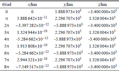
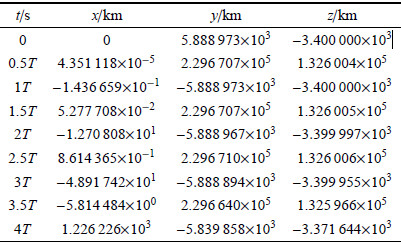
为了验证新模型的数值稳定性和计算精度,将改进后的模型与传统的模型进行了数值对比,积分结果如表1,表2所示. 表1中,$x$方向的误差量级为10$^{-10}$,误差在较小的范围内波动;而表2传统模型的计算结果显示,$x$方向上的误差很大,随着积分时间的增加,误差得不到控制,结果有发散的趋势.因此,改进后的模型积分结果的精度和数值稳定性都大大高于直角坐标动力学方程积分结果的精度和数值稳定性.
表 1(Table 1)

|
表 1
Table 1 |
表 2(Table 2)
|
|
表 2
Table 2 |
5 结论
(1) 改进后的模型体现了轨道动力学与刚体动力 学的联系.在求解单位向量的动力学方程时,将轨道坐标系视为虚拟刚体,轨道坐标系的变化,可视为虚拟刚体相对于惯性空间的姿态变化,可用四元数描述.新模型适用于任意形式的推力或摄动,物理意义更加明显,方便进行轨道设计.
(2) 分别在常值径向力、法向力、切向力以及变摄动力的情况下,对新的动力学方程组进行了验证,与以往的结论相符.同时,新模型的数值稳定性、积分精度都好于惯性系下的轨道动力学模型.
(3) KS变换下,一组物理坐标对应于多组参数坐标,会导致参数混乱. 该模型不具有此弊端;相对于传统的轨道动力学模型,新模型避免了奇异. 当无摄运动时,方程为谐振动方程,可以求得解析解,与KS变换达到的效果一致.
(4) 将传统轨道六要素$\left( {h,e,i,\varOmega ,\omega ,\theta }\right)$转化为新参数$\left( {c_0 ,c_1 ,c_2 ,q_0 ,q_1 ,q_2 ,q_3 }\right)$,其中$\left( {c_0 ,c_1 ,c_2 }\right)$描述航天器在轨道上的位置信息,$\left( {q_0 ,q_1 ,q_2 ,q_3 }\right)$描述轨道在空间的位置信息.
(5) 使用四元数描述轨道的空间方位,体现了轨道动力学和姿态动力学的联系,今后可利用姿态控制的设计方法来设计轨道机动的需用控制力.
参考文献
| [1] |
袁建平, 朱战霞. 空间操作与非开普勒运动. 宇航学报, 2009, 30(1): 42-46 (Yuan Jianping, Zhu Zhanxia. Space operations and non-Keplerian orbit motion. Journal of Astronautics, 2009, 30(1): 42-46 (in Chinese))
|
| [2] |
王萍, 袁建平, 范剑峰. 关于非开普勒轨道的讨论. 宇航学报, 2009, 30(1): 37-41 (Wang Ping, Yuan Jiangping, Fan Jianfeng. A discussion on non-Keplerian orbit. Journal of Astronautics, 2009, 30(1): 37-41 (in Chinese))
|
| [3] |
Stiefel EL, Scheifele G. Linear and Regular Celestial Mechanics. Berlin, New York, Springer-Verlag, 1971: 18-33
|
| [4] |
Vitins M. Kepler motion and gyration. Celestial Mechanics, 1978, 17(2): 173-192
|
| [5] |
曹静, 袁建平, 罗建军. 陀螺进动与强迫进动轨道. 力学学报, 2013, 45(3): 406-411(Cao Jing, Yuan Jianping, Luo Jianjun. Gyroscopic precession and forced precession orbit. Chinese Journal of Theoretical and Applied Mechanics, 2013, 45(3): 406-411 (in Chinese))
|
| [6] |
Peláez J, Hedo JM, de Andrés PR. A special perturbation method in orbital dynamics. Celest Mech Dyn Astr, 2007, 97(2): 131-150
|
| [7] |
Baú G, Bombardelli C, Peláez J. A new set of integrals of motion to propagate the perturbed two-body problem. Celest Mech Dyn Astr, 2013, 116(3): 53-78
|
| [8] |
Junkins JL, Turner JD. On the analogy between orbital dynamics and rigid body dynamics. The Journal of the Astronautical Science, 1979, 17(4): 345-358.
|
| [9] |
Battin RH. An introduction to the mathematics and methods of astrodynamics. AIAA, 2001: 408-415
|
| [10] |
章仁为. 卫星轨道姿态动力学与控制. 北京: 北京航空航天大学出版社, 1998: 157-176 (Zhang Renwei. Satellite Attitude Dynamics and Control. Beijing: Beijing University of Aeronautics and Astronautics Press, 1998: 157-176 (in Chinese))
|
| [11] |
赵育善, 师鹏. 航天器飞行动力学建模理论与方法. 北京: 北京航空航天大学出版社, 2012: 5-27 (Zhao Yushan, Shi Peng. Spacecraft Flight Dyna- mics Modeling Theory and Methods. Beijing: Beijing University of Aeronautics and Astronautics Press, 2012: 5-27 (in Chinese))
|
| [12] |
袁建平, 李俊峰, 和兴锁等. 航天器相对运动轨道动力学. 北京: 中国宇航出版社, 2013: 101-139 (Yuan Jianping, Li Junfeng, He Xingsuo, et al. Relative Orbit Dynamics of Spacecraft. Beijing: China Aerospace Press. 2013: 101-139(in Chinese))
|
| [13] |
刘暾, 赵钧. 空间飞行器动力学. 哈尔滨: 哈尔滨工业大学出版社, 2007: 12-14, 102-114 (Liu Dun, Zhao Jun. Spacecraft Dynamics. Harbin: Harbin Institute of Technology Press. 2007: 12-14, 102-114(in Chinese))
|
| [14] |
肖业伦. 航天器飞行动力学原理. 北京: 宇航出版社, 1995: 26-45 (Xiao Yelun. Spacecraft Dynamics Theory. Beijing: Aerospace Press. 1995: 26-45 (in Chinese))
|
| [15] |
王伟, 袁建平, 罗建军等. 赤道平面J2束缚轨道研究. 中国科学: 物理学, 力学, 天文学, 2013, 43(3): 309-317 (Wang Wei, Yuan Jianping, Luo Jianjun, et al. Anatomy of J2 bounded orbits in equatorial plane. Scientia Sinica Physica, Mechanica & Astronomica, 2013, 43(3): 309-317 (in Chinese))
|
| [16] |
Robert JM, Malcolm M, James B, et al. Survey of highly-non-keplerian orbits with low-thrust propulsion. Journal of Guidance, Control, and Dynamics, 2011, 34(3): 645-666
|
| [17] |
程国采. 四元数法及其应用. 长沙: 国防科技大学出版社, 1991 (Cheng Guocai. Quaternion Theory and Application. Changsha: National University of Defense Technology Press, 1991 (in Chinese))
|
| [18] |
曹静, 袁建平. 空间飞行器轨道相对运动动力学及应用研究.[博士论文]. 西安: 西北工业大学, 2013 (Cao Jing, Yuan Jianping. Kinetics and applied research of spacecraft orbit relative motion.[PhD Thesis]. Xi'an: Northwestern Polytechnical University. 2013 (in Chinese))
|
AN IMPROVED MODEL OF ORBITAL DYNAMICS
Yang Mengjie

, Yuan Jianping
National Key Laboratory of Aerospace Flight Dynamics, Northwestern Polytechnical University, Xi'an 710072, China
Abstract: The radius vector of spacecraft can be decomposed into the product of the mold and the unit vector. Using this property, the traditional orbital dynamics equation can be transformed into two equations which describe the mold's and direction's motions separately. The mold's equation can be converted to a linear equation without singularity by introducing the inverse of the mold; and using the variation of constants method, the linear equation can be reduced to one-order. As for the direction's equation, the quaternion description is suitable. This equation can be completely solved. Through the above handling methods, we obtain a new orbital dynamic model which contains seven equations. In the sense of the virtual time, the angular velocity of the spacecraft depends only on the normal force. This new orbital model is applicable to any form of thrust or perturbation. At the same time, we get seven new stable variables which completely equivalent to the kepler elements. And the transforming relationship has been established. In the end of this article, we verify the accuracy and applicability of the new model in the cases of constant and variable thrusts.
Key words:
orbital model continuous thrust orbital maneuvering changing constant quaternion
 2015, Vol. 47